Plot contours

This tutorial shows different commands for plotting data contours on meshes.

PyDPF-Core has a variety of plotting methods for generating 3D plots with Python. These methods use VTK and leverage the PyVista library.

Load data to plot

Load a result file in a model

import ansys.dpf.core as dpf
from ansys.dpf.core import examples, operators as ops

result_file_path_1 = examples.download_piston_rod()
model_1 = dpf.Model(data_sources=result_file_path_1)

Extract data for the contour

For more information about extracting results from a result file, see the Import Data tutorials section.

Note

Only the elemental or nodal locations are supported for plotting.

Here, we choose to plot the XX component of the stress tensor.

stress_XX_op = ops.result.stress_X(data_sources=model_1)

# The default behavior is to return data as ElementalNodal
print(stress_XX_op.eval())

DPF stress(s)Fields Container
  with 1 field(s)
  defined on labels: time

  with:
  - field 0 {time:  3} with Nodal location, 1 components and 33337 entities.

Request the stress in a nodal location (the default ElementalNodal location is not supported for plotting). We define the new location using the operator input. Another option would be using the to_nodal_fc averaging operator on the output of the stress operator.

stress_XX_op.inputs.requested_location(dpf.locations.nodal)
stress_XX_fc = stress_XX_op.eval()

Extract the mesh

meshed_region_1 = model_1.metadata.meshed_region

Plot a contour of a single field

There are three methods to plot a single Field:

• Field.plot()

• MeshedRegion.plot() with the field as argument

• DpfPlotter with add_field() (more performant)

Get a single field from the FieldsContainer.

stress_XX = stress_XX_fc[0]

Plot using Field.plot()

If the Field does not have an associated mesh support (see Field.meshed_region), provide a mesh with the meshed_region argument.

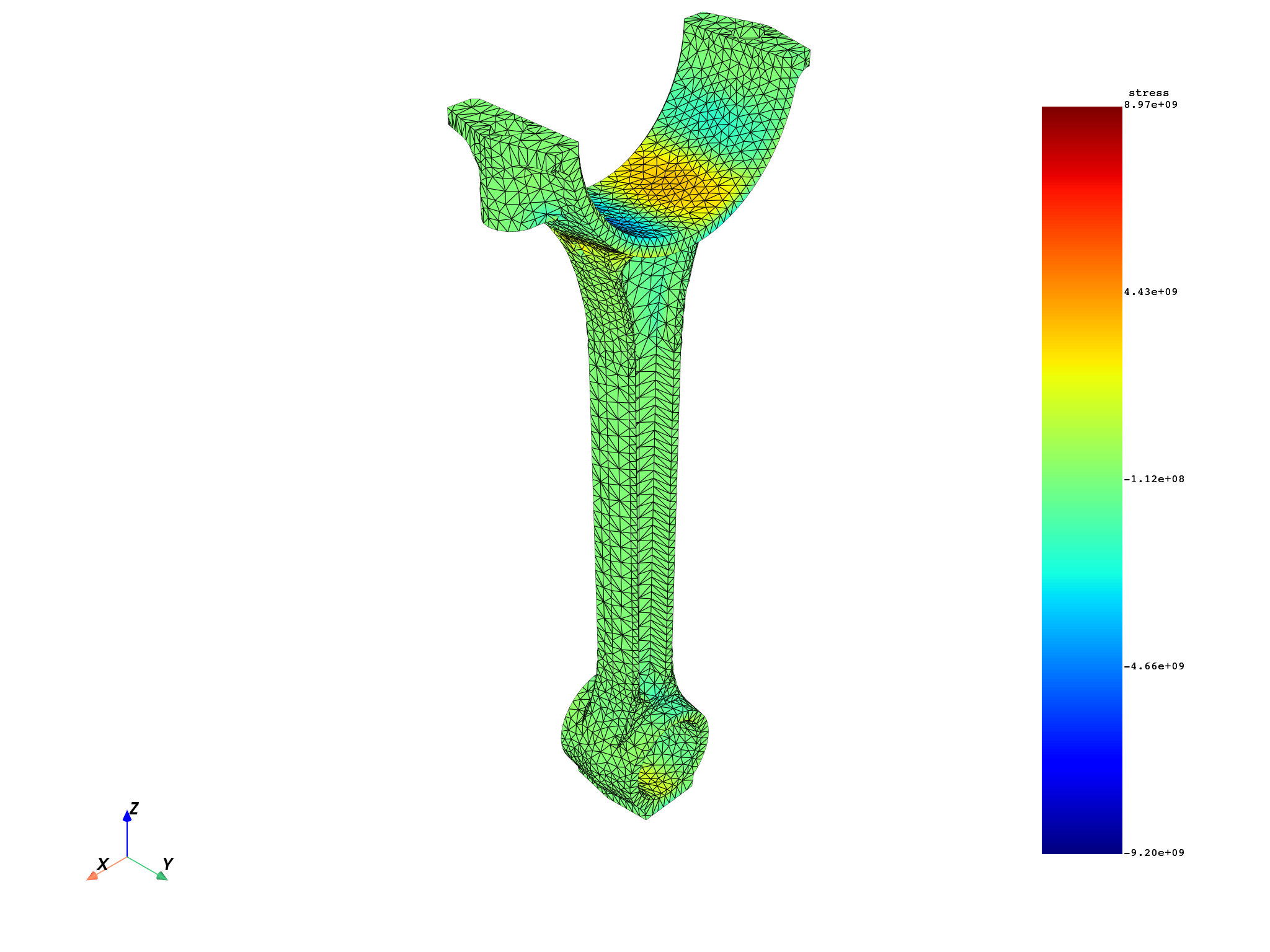
stress_XX.plot(meshed_region=meshed_region_1)

(None, <pyvista.plotting.plotter.Plotter object at 0x0000013BD4F67110>)

Plot using MeshedRegion.plot()

Use the field_or_fields_container argument to pass the field.

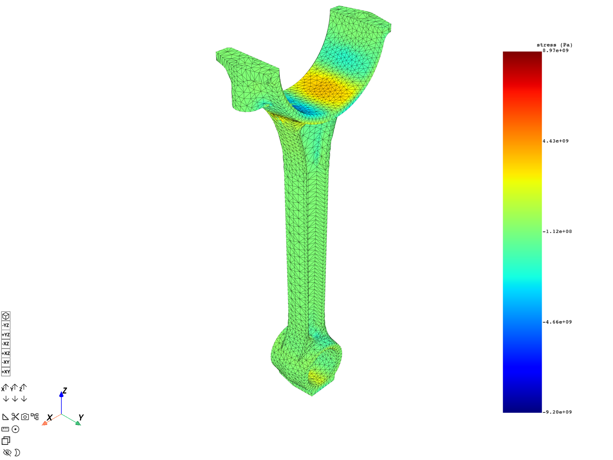
meshed_region_1.plot(field_or_fields_container=stress_XX)

(None, <pyvista.plotting.plotter.Plotter object at 0x0000013BD52469D0>)

Plot using DpfPlotter

1. Create an instance of DpfPlotter.

2. Add the field using add_field(). If the field has no associated mesh support, provide a mesh with the meshed_region argument.

3. Render and show the figure using show_figure().

You can also first call add_mesh() to add the mesh and then call add_field() without the meshed_region argument.

plotter_1 = dpf.plotter.DpfPlotter()
plotter_1.add_field(field=stress_XX, meshed_region=meshed_region_1)
plotter_1.show_figure()

([], <pyvista.plotting.plotter.Plotter object at 0x0000013BD4CFFBD0>)

Plot a contour of multiple fields

Prepare a collection of fields

Warning

The fields should not have conflicting data — you cannot build a contour for two fields with two different sets of data for the same mesh entities (intersecting scopings). These methods are therefore not available for a collection of fields varying across time, or for different shell layers of the same elements.

Here we split the field for XX stress based on material to get a collection of fields with non-conflicting associated mesh entities.

We use the split_fields operator together with the split_mesh operator. For MAPDL results, a split on material is equivalent to a split on bodies.

fields = (
    ops.mesh.split_fields(
        field_or_fields_container=stress_XX_fc,
        meshes=ops.mesh.split_mesh(mesh=meshed_region_1, property="mat"),
    )
).eval()
print(fields)

DPF  Fields Container
  with 2 field(s)
  defined on labels: body mat time

  with:
  - field 0 {mat:  1, body:  1, time:  3} with Nodal location, 1 components and 17281 entities.
  - field 1 {mat:  2, body:  2, time:  3} with Nodal location, 1 components and 17610 entities.

Plot the contour using FieldsContainer.plot()

Use FieldsContainer.plot().

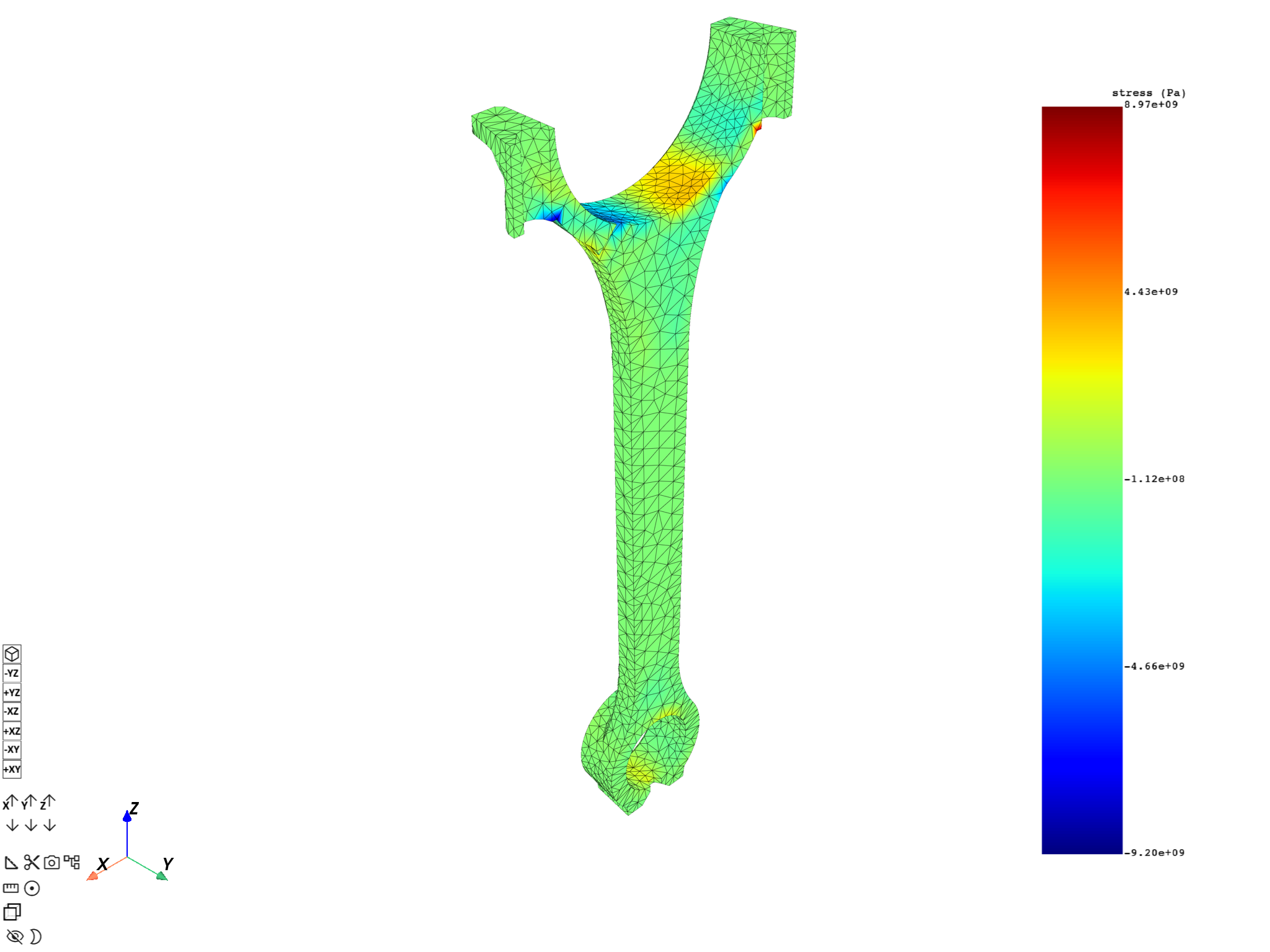
fields.plot()

([], <pyvista.plotting.plotter.Plotter object at 0x0000013BD45525D0>)

The label_space argument provides further field filtering capabilities.

fields.plot(label_space={"mat": 1})

([], <pyvista.plotting.plotter.Plotter object at 0x0000013BD4E028D0>)

Plot the contour using MeshedRegion.plot()

Use the field_or_fields_container argument.

meshed_region_1.plot(field_or_fields_container=fields)

(None, <pyvista.plotting.plotter.Plotter object at 0x0000013BD44C0110>)

Plot the contour using DpfPlotter

Add each field individually using add_field().

plotter_2 = dpf.plotter.DpfPlotter()
plotter_2.add_field(field=fields[0])
plotter_2.add_field(field=fields[1])
plotter_2.show_figure()

([], <pyvista.plotting.plotter.Plotter object at 0x0000013BD49C4BD0>)