Plot contours

This tutorial shows different commands for plotting data contours on meshes.

PyDPF-Core has a variety of plotting methods for generating 3D plots with Python. These methods use VTK and leverage the PyVista library.

Download tutorial as Python script Download tutorial as Jupyter notebook

Load data to plot

Load a result file in a model

For this tutorial, we use mesh information and data from a case available in the Examples module. For more information on how to import your own result file in DPF, see the Import Data tutorials section.

# Import the ``ansys.dpf.core`` module
import ansys.dpf.core as dpf
# Import the examples module
from ansys.dpf.core import examples
# Import the operators module
from ansys.dpf.core import operators as ops

# Define the result file path
result_file_path_1 = examples.download_piston_rod()

# Create a model from the result file
model_1 = dpf.Model(data_sources=result_file_path_1)

Extract data for the contour

Extract data for the contour. For more information about extracting results from a result file, see the Import Data tutorials section.

Note

Only the ‘elemental’ or ‘nodal’ locations are supported for plotting.

Here, we choose to plot the XX component of the stress tensor.

# Get the stress operator for component XX
stress_XX_op = ops.result.stress_X(data_sources=model_1)

# The default behavior of the operator is to return data as *'ElementalNodal'*
print(stress_XX_op.eval())

DPF stress(s)Fields Container
  with 1 field(s)
  defined on labels: time 

  with:
  - field 0 {time:  3} with Nodal location, 1 components and 33337 entities.

We must request the stress in a ‘nodal’ location as the default ‘ElementalNodal’ location for the stress results is not supported for plotting.

There are different ways to change the location. Here, we define the new location using the input of the stress operator. Another option would be using an averaging operator on the output of the stress operator, like the to_nodal_fc operator

# Define the desired location as an input of the stress operator
stress_XX_op.inputs.requested_location(dpf.locations.nodal)

# Get the output
stress_XX_fc = stress_XX_op.eval()

The output if a collection of fields, a FieldsContainer.

Extract a mesh

Here we simply get the MeshedRegion object of the model, but any other MeshedRegion works.

# Extract the mesh
meshed_region_1 = model_1.metadata.meshed_region

Plot a contour of a single field

To plot a single Field, you can use:

• the Field.plot() method

• the MeshedRegion.plot() method with the field as argument

• the DpfPlotter class and its add_field() method

Hint

Using the DpfPlotter class is more performant than using the Field.plot() method

Field.plot()

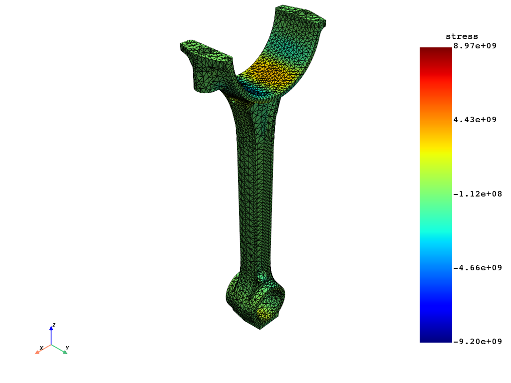
First, get a Field from the stress results FieldsContainer. Then, use the Field.plot() method [1]. If the Field does not have an associated mesh support (see Field.meshed_region), you must use the meshed_region argument and provide a mesh.

# Get a single field
stress_XX = stress_XX_fc[0]

# Plot the contour on the mesh
stress_XX.plot(meshed_region=meshed_region_1)

(None, <pyvista.plotting.plotter.Plotter at 0x1d732232cf0>)

MeshedRegion.plot()

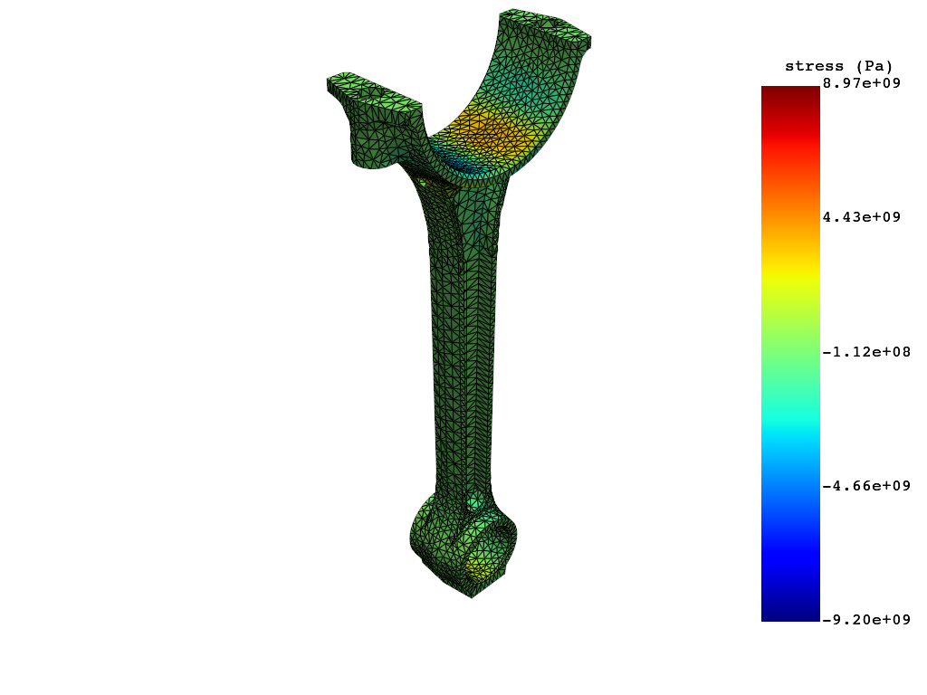
Use the MeshedRegion.plot() method [1]. You must use the ‘field_or_fields_container’ argument and give the Field or the FieldsContainer containing the stress results data.

# Plot the mesh with the stress field contour
meshed_region_1.plot(field_or_fields_container=stress_XX)

(None, <pyvista.plotting.plotter.Plotter at 0x1d708306780>)

DpfPlotter

First create an instance of DpfPlotter [2]. Then, add the Field to the scene using the add_field() method. If the Field does not have an associated mesh support (see Field.meshed_region), you must use the ‘meshed_region’ argument and provide a mesh.

To render and show the figure based on the current state of the plotter object, use the show_figure() method.

# Create a DpfPlotter instance
plotter_1 = dpf.plotter.DpfPlotter()

# Add the field to the scene, here with an explicitly associated mesh
plotter_1.add_field(field=stress_XX, meshed_region=meshed_region_1)

# Display the scene
plotter_1.show_figure()

(None, <pyvista.plotting.plotter.Plotter at 0x1d737fa0a10>)

You can also first use the add_mesh() method to add the mesh to the scene and then use add_field() without the meshed_region argument.

Plot a contour of multiple fields

Prepare a collection of fields

Warning

The fields should not have conflicting data, meaning you cannot build a contour for two fields with two different sets of data for the same mesh entities (intersecting scopings).

This means the following methods are for example not available for a collection made of the same field varying across time, or a collection of fields for different shell layers of the same elements.

Here we split the field for XX stress based on material to get a collection of fields with non-conflicting associated mesh entities.

We use the split_fields operator to split the field based on the result of the split_mesh operator. The split_mesh operator returns a MeshesContainer with meshes labeled according to the criterion for the split. In our case, the split criterion is the material ID.

# Split the field based on material property
fields = (
    ops.mesh.split_fields(
        field_or_fields_container=stress_XX_fc,
        meshes=ops.mesh.split_mesh(mesh=meshed_region_1, property="mat"),
    )
).eval()

# Show the result
print(fields)

DPF  Fields Container
  with 2 field(s)
  defined on labels: body mat time 

  with:
  - field 0 {mat:  1, body:  1, time:  3} with Nodal location, 1 components and 17281 entities.
  - field 1 {mat:  2, body:  2, time:  3} with Nodal location, 1 components and 17610 entities.

For MAPDL results the split on material is equivalent to a split on bodies, hence the two equivalent labels.

Plot the contour

To plot a contour for multiple Field objects, you can use:

• the FieldsContainer.plot() method if the fields are in a collection

• the MeshedRegion.plot() method with the field collection as argument

• the DpfPlotter class and several calls to its add_field() method

Hint

Using the DpfPlotter class is more performant than using the Field.plot() method

FieldsContainer.plot()

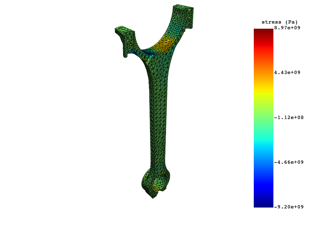
Use the FieldsContainer.plot() method [1].

# Plot the contour for all fields in the collection
fields.plot()

(None, <pyvista.plotting.plotter.Plotter at 0x1d737fba780>)

The label_space argument provides further field filtering capabilities.

# Plot the contour for ``mat`` 1 only
fields.plot(label_space={"mat":1})

(None, <pyvista.plotting.plotter.Plotter at 0x1d72d4577a0>)

MeshedRegion.plot()

Use the MeshedRegion.plot() method [1]. You must use the ‘field_or_fields_container’ argument and give the Field or the FieldsContainer containing the stress results data.

# Plot the mesh with the stress field contours
meshed_region_1.plot(field_or_fields_container=fields)

(None, <pyvista.plotting.plotter.Plotter at 0x1d737fbb140>)

DpfPlotter

First create an instance of DpfPlotter [2]. Then, add each Field to the scene using the add_field() method. If the Field does not have an associated mesh support (see Field.meshed_region), you must use the ‘meshed_region’ argument and provide a mesh.

To render and show the figure based on the current state of the plotter object, use the show_figure() method.

# Create a DpfPlotter instance
plotter_1 = dpf.plotter.DpfPlotter()

# Add each field to the scene
plotter_1.add_field(field=fields[0])
plotter_1.add_field(field=fields[1])

# Display the scene
plotter_1.show_figure()

(None, <pyvista.plotting.plotter.Plotter at 0x1d72d4a2510>)

Footnotes

[1] (1,2,3,4)

The DpfPlotter displays the mesh with edges, lighting and axis widget enabled by default. You can pass additional PyVista arguments to all plotting methods to change the default behavior (see options for pyvista.plot()), such as:

model_1.plot(title="Mesh",
             text="this is a mesh",  # Adds the given text at the bottom of the plot
             off_screen=True,
             screenshot="mesh_plot_1.png",  # Save a screenshot to file with the given name
             window_size=[450,350])
# Notes:
# - To save a screenshot to file, use "screenshot=figure_name.png" ( as well as "notebook=False" if on a Jupyter notebook).
# - The "off_screen" keyword only works when "notebook=False". If "off_screen=True" the plot is not displayed when running the code.

(None, <pyvista.plotting.plotter.Plotter at 0x1d737fbab70>)

[2] (1,2)

The DpfPlotter is currently based on PyVista. That means that PyVista must be installed. The DPF plotter also passes additional parameters to the PyVista plotter (arguments supported by the version of PyVista installed). More information about available additional arguments is available at pyvista.plot().