Plot a graph using matplotlib#
This tutorial explains how to plot a graph with data from DPF using matplotlib.
The current DpfPlotter module does not allow to plot graphs. Instead, you need to import the
matplotlib library to plot graphs with PyDPF-Core.
Download tutorial as Python script
Download tutorial as Jupyter notebook
There is a large range of graphs you can plot. Here, we showcase:
Result along a path#
In this tutorial, we plot the norm of the displacement along a custom path represented by a Line.
For more information about how to create a custom geometric object,
see the ref_tutorials_plot_on_custom_geometry tutorial.
We first need to get the data of interest, then create a custom Line geometry for the path.
We then map the result on the path, and finally create a 2D graph.
Extract the data#
First, extract the data from a result file or create some from scratch.
For this tutorial we use a case available in the Examples module.
For more information on how to import your own result file in DPF,
or on how to create data from user input in PyDPF-Core,see
the Import Data tutorials section.
# Import the ``ansys.dpf.core`` module
import ansys.dpf.core as dpf
# Import the examples module
from ansys.dpf.core import examples
# Import the operators module
from ansys.dpf.core import operators as ops
# Import the geometry module
from ansys.dpf.core import geometry as geo

# Import the ``matplotlib.pyplot`` module
import matplotlib.pyplot as plt

# Download and get the path to an example result file
result_file_path_1 = examples.find_static_rst()

# Create a model from the result file
model_1 = dpf.Model(data_sources=result_file_path_1)
We then extract the result of interest for the graph. In this tutorial, we want the norm of the displacement field at the last step.
# Get the nodal displacement field at the last simulation step (default)
disp_results_1 = model_1.results.displacement.eval()

# Get the norm of the displacement field
norm_disp = ops.math.norm_fc(fields_container=disp_results_1).eval()
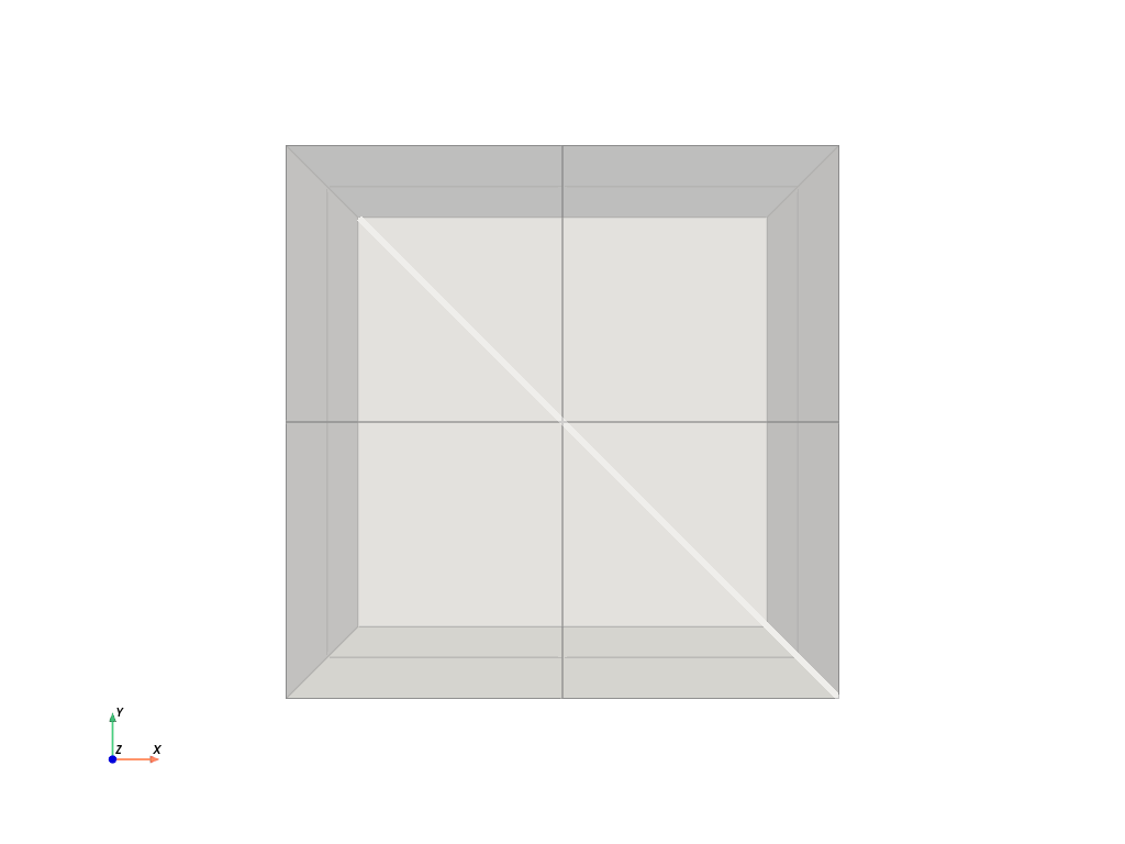
Define the path#
Create a path as a Line passing through the diagonal of the mesh.
# Create a discretized line for the path
line_1 = geo.Line(coordinates=[[0.0, 0.06, 0.0], [0.03, 0.03, 0.03]], n_points=50)
# Plot the line on the original mesh
line_1.plot(mesh=model_1.metadata.meshed_region)
Map the data on the path#
Map the displacement norm field to the Line using the on_coordinates mapping operator.
This operator interpolates field values at given node coordinates, using element shape functions.
It takes as input a FieldsContainer of data, a 3D vector Field of coordinates to interpolate at,
and an optional MeshedRegion to use for element shape functions if the first Field in the data
provided does not have an associated meshed support.
# Interpolate the displacement norm field at the nodes of the custom path
disp_norm_on_path_fc: dpf.FieldsContainer = ops.mapping.on_coordinates(
    fields_container=norm_disp,
    coordinates=line_1.mesh.nodes.coordinates_field,
).eval()
# Extract the only field in the collection obtained
disp_norm_on_path: dpf.Field = disp_norm_on_path_fc[0]
print(disp_norm_on_path)
DPF displacement_1.s Field
  Location: Nodal
  Unit: m
  50 entities
  Data: 1 components and 50 elementary data

  IDs                   data(m)
  ------------          ----------
  1                     1.481537e-08

  2                     1.451810e-08

  3                     1.421439e-08

  ...
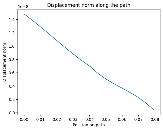
Plot the graph#
Plot a graph of the norm of the displacement field along the path using the matplotlib library.
To get the parametric coordinates of the nodes along the line and use them as X-axis,
you can use the Line.path property.
It gives the 1D array of parametric coordinates of the nodes of the line along the line.
The values in the displacement norm field are in the same order as the parametric coordinates because the mapping operator orders output data the same as the input coordinates.
# Get the field of parametric coordinates along the path for the X-axis
line_coordinates = line_1.path

# Define the curve to plot
plt.plot(line_coordinates, disp_norm_on_path.data)

# Add titles to the axes and the graph
plt.xlabel("Position on path")
plt.ylabel("Displacement norm")
plt.title("Displacement norm along the path")

# Display the graph
plt.show()
Transient data#
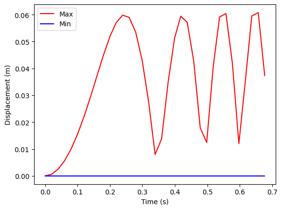
In this tutorial, we plot the minimum and maximum displacement norm over time for a transient analysis. For more information about using PyDPF-Core with a transient analysis, see the Transient analysis examples examples.
We first need to create data for the Y-axis, and then format the time information of the model for the X-axis, to finally create a 2D graph using both.
Prepare data#
First, extract the data from a transient result file or create some from scratch.
For this tutorial we use a transient case available in the Examples module.
For more information on how to import your own result file in DPF,
or on how to create data from user input in PyDPF-Core, see
the Import Data tutorials section.
# Import the ``ansys.dpf.core`` module
import ansys.dpf.core as dpf
# Import the examples module
from ansys.dpf.core import examples
# Import the operators module
from ansys.dpf.core import operators as ops

# Import the ``matplotlib.pyplot`` module
import matplotlib.pyplot as plt

# Download and get the path to an example transient result file
result_file_path_2 = examples.download_transient_result()

# Create a model from the result file
model_2 = dpf.Model(data_sources=result_file_path_2)

# Check the model is transient with its ``TimeFreqSupport``
print(model_2.metadata.time_freq_support)
DPF  Time/Freq Support:
  Number of sets: 35
Cumulative     Time (s)       LoadStep       Substep
1              0.000000       1              1
2              0.019975       1              2
3              0.039975       1              3
4              0.059975       1              4
5              0.079975       1              5
6              0.099975       1              6
7              0.119975       1              7
8              0.139975       1              8
9              0.159975       1              9
10             0.179975       1              10
11             0.199975       1              11
12             0.218975       1              12
13             0.238975       1              13
14             0.258975       1              14
15             0.278975       1              15
16             0.298975       1              16
17             0.318975       1              17
18             0.338975       1              18
19             0.358975       1              19
20             0.378975       1              20
21             0.398975       1              21
22             0.417975       1              22
23             0.437975       1              23
24             0.457975       1              24
25             0.477975       1              25
26             0.497975       1              26
27             0.517975       1              27
28             0.537550       1              28
29             0.557253       1              29
30             0.577118       1              30
31             0.597021       1              31
32             0.616946       1              32
33             0.636833       1              33
34             0.656735       1              34
35             0.676628       1              35
We then extract the result of interest for the graph. In this tutorial, we want the maximum and minimum displacement norm over the field at each time step.
First extract the displacement field for every time step.
# Get the displacement at all time steps
disp_results_2: dpf.FieldsContainer = model_2.results.displacement.on_all_time_freqs.eval()
Next, get the minimum and maximum of the norm of the displacement at each time step using the min_max_fc operator.
# Instantiate the min_max operator and give the output of the norm operator as input
min_max_op = ops.min_max.min_max_fc(fields_container=ops.math.norm_fc(disp_results_2))

# Get the field of maximum values at each time-step
max_disp: dpf.Field = min_max_op.outputs.field_max()
print(max_disp)

# Get the field of minimum values at each time-step
min_disp: dpf.Field = min_max_op.outputs.field_min()
print(min_disp)
DPF displacement_0.s Field
  Location: Nodal
  Unit: m
  35 entities
  Data: 1 components and 35 elementary data

  IDs                   data(m)
  ------------          ----------
  0                     0.000000e+00

  1                     6.267373e-04

  2                     2.509401e-03

  ...


DPF displacement_0.s Field
  Location: Nodal
  Unit: m
  35 entities
  Data: 1 components and 35 elementary data

  IDs                   data(m)
  ------------          ----------
  0                     0.000000e+00

  1                     0.000000e+00

  2                     0.000000e+00

  ...
The operator already outputs fields where data points are associated to time-steps.
Prepare time values#
The time or frequency information associated to DPF objects is stored in TimeFreqSupport objects.
You can use the TimeFreqSupport of a Field with location time_freq to retrieve the time or
frequency values associated to the entities mentioned in its scoping.
Here the fields are on all time-steps, so we can simply get the list of all time values without filtering.
# Get the field of time values
time_steps_1: dpf.Field = disp_results_2.time_freq_support.time_frequencies

# Print the time values
print(time_steps_1)
DPF  Field
  Location: timefrq_sets
  Unit: s
  1 entities
  Data: 1 components and 35 elementary data

  TimeFreq_steps
  IDs                   data(s)
  ------------          ----------
  1                     0.000000e+00
                        1.997500e-02
                        3.997500e-02
                        ...
The time values associated to time-steps are given in a Field.
To use it in the graph you need to extract the data of the Field as an array.
# Get the time values
time_data = time_steps_1.data
print(time_data)
[0.         0.019975   0.039975   0.059975   0.079975   0.099975
 0.119975   0.139975   0.159975   0.179975   0.199975   0.218975
 0.238975   0.258975   0.278975   0.298975   0.318975   0.338975
 0.358975   0.378975   0.398975   0.417975   0.437975   0.457975
 0.477975   0.497975   0.517975   0.53754972 0.55725277 0.57711786
 0.59702054 0.61694639 0.63683347 0.65673452 0.67662783]
Plot the graph#
Plot a graph of the minimum and maximum displacement over time using the matplotlib library.
Use the unit property of the fields to properly label the axes.
# Define the plot figure
plt.plot(time_data, max_disp.data, "r", label="Max")
plt.plot(time_data, min_disp.data, "b", label="Min")

# Add axis labels and legend
plt.xlabel(f"Time ({time_steps_1.unit})")
plt.ylabel(f"Displacement ({max_disp.unit})")
plt.legend()

# Display the graph
plt.show()