RBF-based workflow mapping

Generate a reusable workflow for mapping results using Radial Basis Function (RBF) filters.

This tutorial demonstrates how to use the prepare_mapping_workflow operator to generate a reusable Workflow that maps results between meshes with different topologies using RBF filters.

Unlike shape-function interpolation (used by on_coordinates and on_reduced_coordinates), RBF-based mapping can transfer data between non-conforming meshes where element boundaries do not align. It evaluates target values by weighting surrounding source nodes based on distance. The filter radius acts like a standard deviation in Gaussian weighting—small radii capture local gradients while larger radii produce smoother trends. The optional influence box limits the spatial search window as a computational optimization.

The resulting workflow accepts a source field and returns the interpolated target field; it can be reused for multiple field types without repeating the setup step.

Import modules and load the model

Import the required modules and load a result file.

# Import the ``ansys.dpf.core`` module
# Import Matplotlib for plotting
import matplotlib.pyplot as plt

from ansys.dpf import core as dpf

# Import the examples and operators modules
from ansys.dpf.core import examples, operators as ops

Load model

Download the crankshaft result file and create a Model object.

result_file = examples.download_crankshaft()
model = dpf.Model(data_sources=result_file)
print(model)

DPF Model
------------------------------
Static analysis
Unit system: MKS: m, kg, N, s, V, A, degC
Physics Type: Mechanical
Available results:
     -  node_orientations: Nodal Node Euler Angles
     -  displacement: Nodal Displacement
     -  velocity: Nodal Velocity
     -  acceleration: Nodal Acceleration
     -  reaction_force: Nodal Force
     -  stress: ElementalNodal Stress
     -  elemental_volume: Elemental Volume
     -  stiffness_matrix_energy: Elemental Energy-stiffness matrix
     -  artificial_hourglass_energy: Elemental Hourglass Energy
     -  kinetic_energy: Elemental Kinetic Energy
     -  co_energy: Elemental co-energy
     -  incremental_energy: Elemental incremental energy
     -  thermal_dissipation_energy: Elemental thermal dissipation energy
     -  elastic_strain: ElementalNodal Strain
     -  elastic_strain_eqv: ElementalNodal Strain eqv
     -  element_orientations: ElementalNodal Element Euler Angles
     -  structural_temperature: ElementalNodal Structural temperature
------------------------------
DPF  Meshed Region:
  69762 nodes
  39315 elements
  Unit: m
  With solid (3D) elements
------------------------------
DPF  Time/Freq Support:
  Number of sets: 3
Cumulative     Time (s)       LoadStep       Substep
1              1.000000       1              1
2              2.000000       1              2
3              3.000000       1              3

Define the input support

The input support is the mesh from which results will be mapped. Use bounding_box to inspect the spatial extent of the crankshaft before choosing a filter radius.

input_mesh = model.metadata.meshed_region
bb_data = input_mesh.bounding_box.data[0]  # [xmin, ymin, zmin, xmax, ymax, zmax]
print(
    f"Bounding box: x=[{bb_data[0]:.4f}, {bb_data[3]:.4f}] "
    f"y=[{bb_data[1]:.4f}, {bb_data[4]:.4f}] "
    f"z=[{bb_data[2]:.4f}, {bb_data[5]:.4f}] m"
)

Bounding box: x=[-0.0250, 0.0350] y=[-0.0250, 0.0250] z=[-0.0720, 0.0500] m

Define the output support

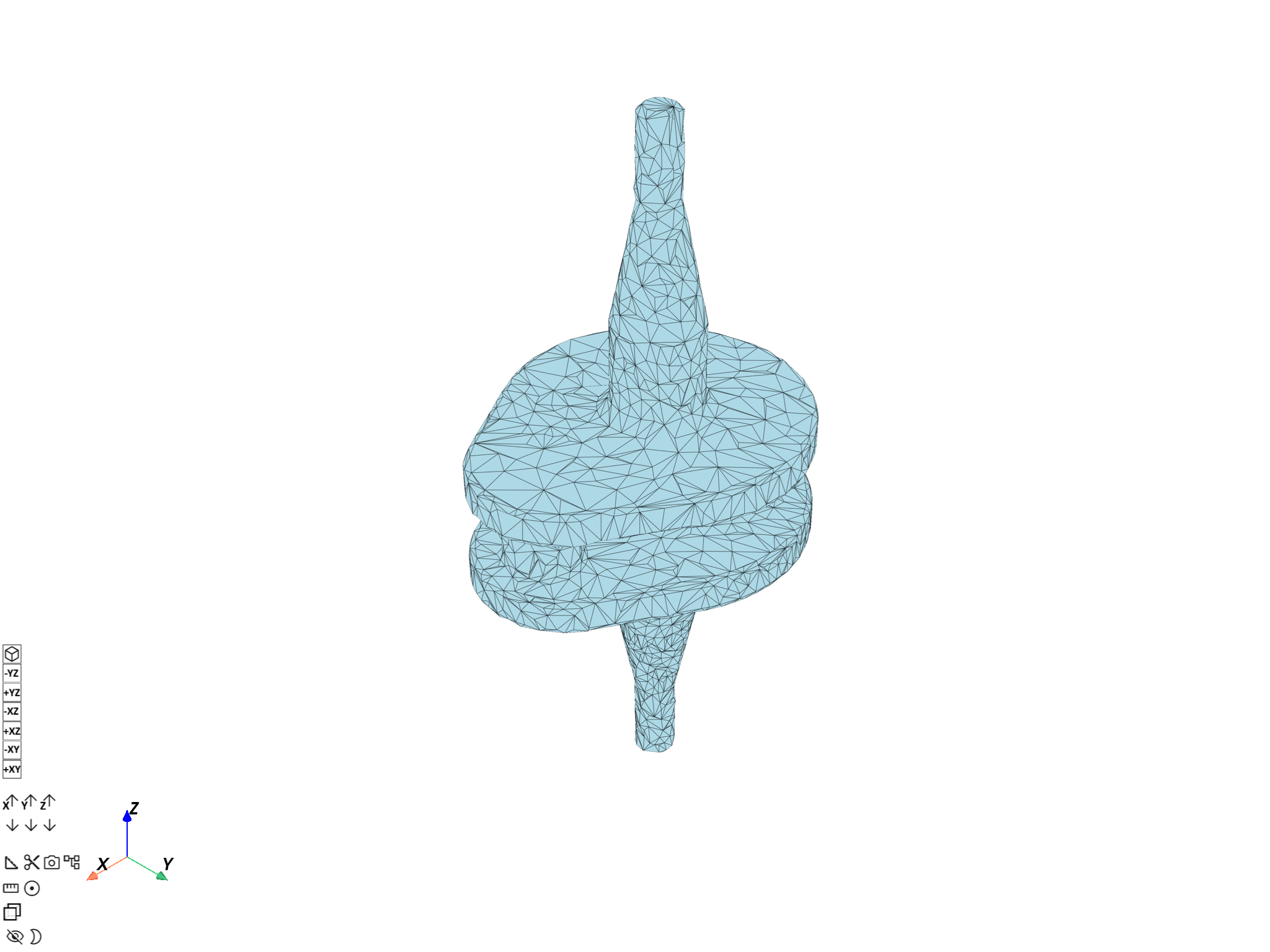
The output support is the target mesh onto which results will be mapped. To demonstrate RBF mapping between non-conforming meshes with genuinely different topologies, the output mesh is built in two steps:

1. Extract the external surface of the crankshaft using the skin operator.

2. Decimate that surface to ~30 % of its original faces using decimate_mesh, which produces a coarser triangulated mesh.

This gives a source (solid, hexahedral) / target (surface, triangulated) pair with entirely different topology — exactly the scenario RBF-based mapping is designed for.

skin_mesh = ops.mesh.skin(mesh=input_mesh).outputs.mesh()
output_mesh = ops.mesh.decimate_mesh(
    mesh=skin_mesh,
    preservation_ratio=0.3,
).outputs.mesh()

print(
    f"Source mesh:          {input_mesh.nodes.n_nodes} nodes, {input_mesh.elements.n_elements} elements (solid)"
)
print(
    f"Skin mesh:            {skin_mesh.nodes.n_nodes} nodes, {skin_mesh.elements.n_elements} elements (surface)"
)
print(
    f"Decimated target mesh:{output_mesh.nodes.n_nodes} nodes, {output_mesh.elements.n_elements} elements (triangles)"
)
input_mesh.plot(title="Source mesh (crankshaft solid)")
output_mesh.plot(title="Target mesh (decimated surface)")

• 
• 

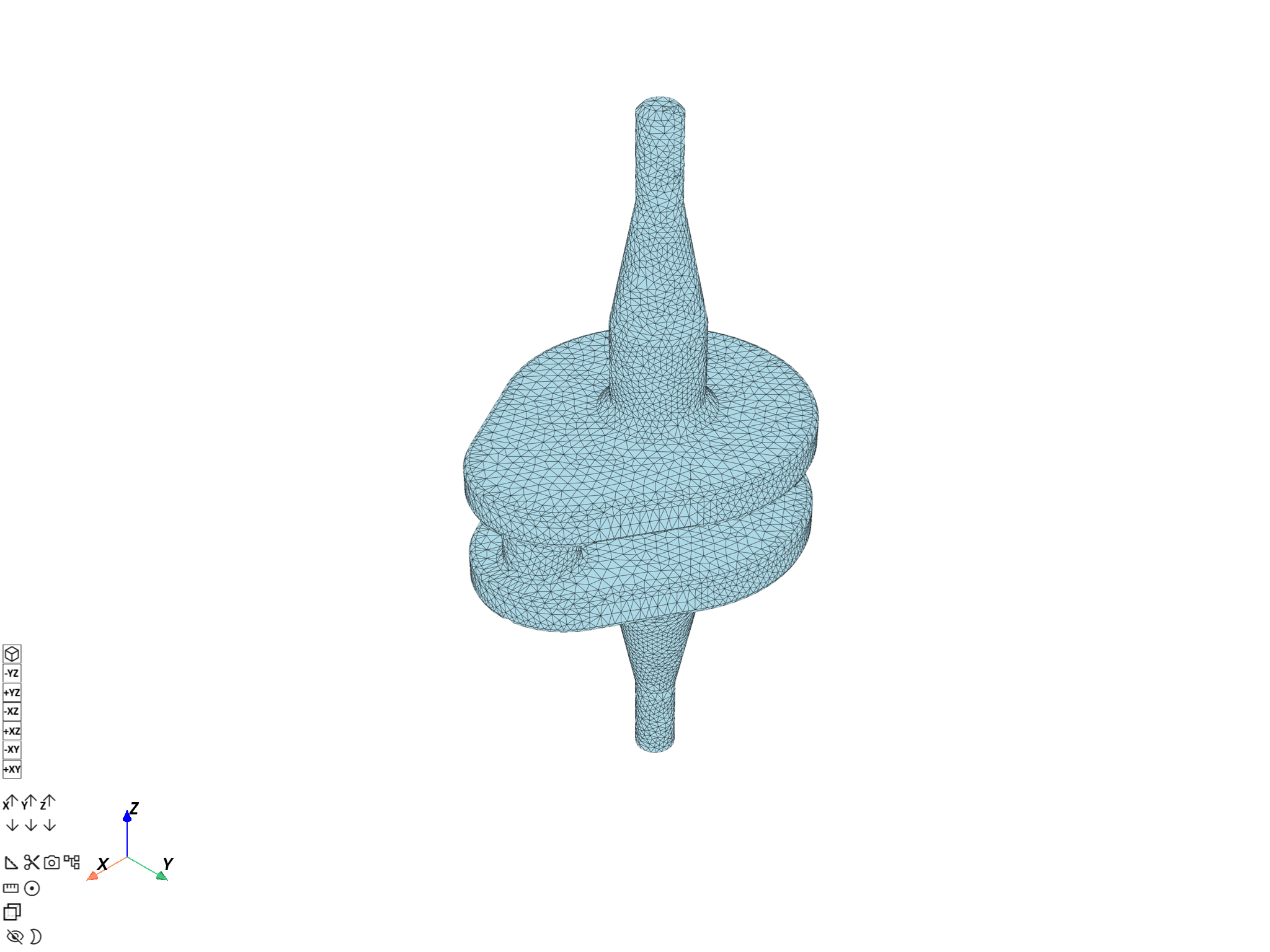
Source mesh:          69762 nodes, 39315 elements (solid)
Skin mesh:            32922 nodes, 16460 elements (surface)
Decimated target mesh:2471 nodes, 4938 elements (triangles)

([], <pyvista.plotting.plotter.Plotter object at 0x0000021582F074D0>)

Prepare the mapping workflow

Call prepare_mapping_workflow to build an RBF-based Workflow that maps fields from the input support to the output support. The filter radius controls the RBF smoothing scale. A value of 5 mm (0.005 m) is appropriate for the crankshaft which spans ~60 mm in its narrowest dimension.

filter_radius = 0.005

prepare_op = ops.mapping.prepare_mapping_workflow(
    input_support=input_mesh,
    output_support=output_mesh,
    filter_radius=filter_radius,
)
mapping_workflow = prepare_op.eval()
mapping_workflow.progress_bar = False
print("Generated mapping workflow:")
print(mapping_workflow)

Generated mapping workflow:
DPF Workflow:
  with 3 operator(s): apply_mapping, make_rbf_mapper, default_value
  the exposed input pins are: optional_target_support, source
  the exposed output pins are: target

Examine the generated workflow

The workflow exposes a "source" input pin and a "target" output pin.

print("Workflow operator names:")
for i, name in enumerate(mapping_workflow.operator_names):
    print(f"  {i + 1}. {name}")

Workflow operator names:
  1. apply_mapping
  2. make_rbf_mapper
  3. default_value

Map displacement using the workflow

Connect a displacement field to the workflow "source" pin and retrieve the interpolated result from the "target" pin.

displacement_fc = model.results.displacement.eval()
displacement_field = displacement_fc[0]
input_mesh.plot(field_or_fields_container=displacement_fc, title="Source displacement (crankshaft)")

input_pin_name = "source"
output_pin_name = "target"

mapping_workflow.connect(pin_name=input_pin_name, inpt=displacement_field)
mapped_displacement_field = mapping_workflow.get_output(
    pin_name=output_pin_name,
    output_type=dpf.types.field,
)
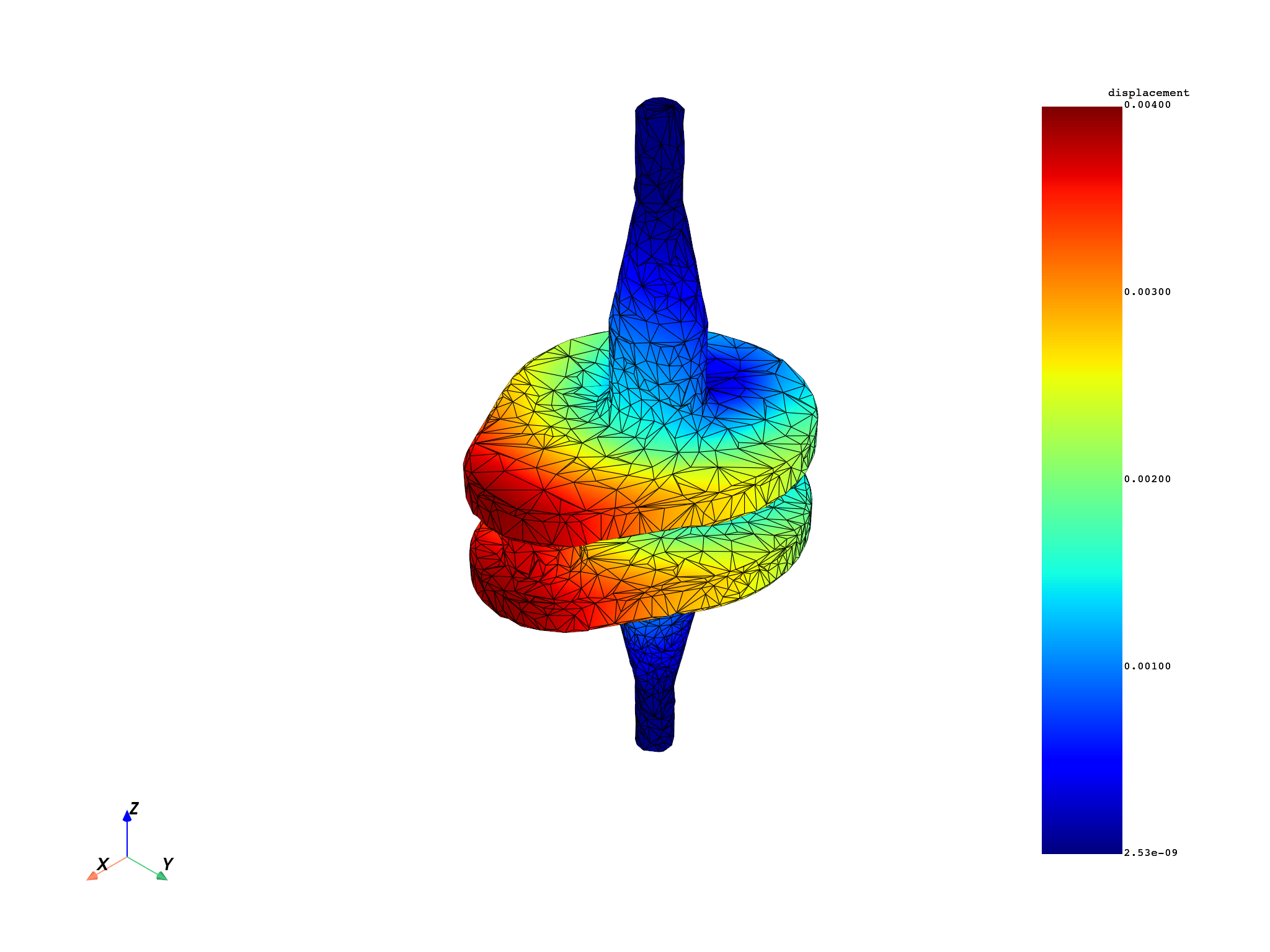
output_mesh.plot(
    field_or_fields_container=mapped_displacement_field,
    title="Mapped displacement on decimated surface",
)

print(f"Source field:  {len(displacement_field.data)} entities (solid nodes)")
print(f"Mapped field:  {len(mapped_displacement_field.data)} entities (surface nodes)")

• 
• 

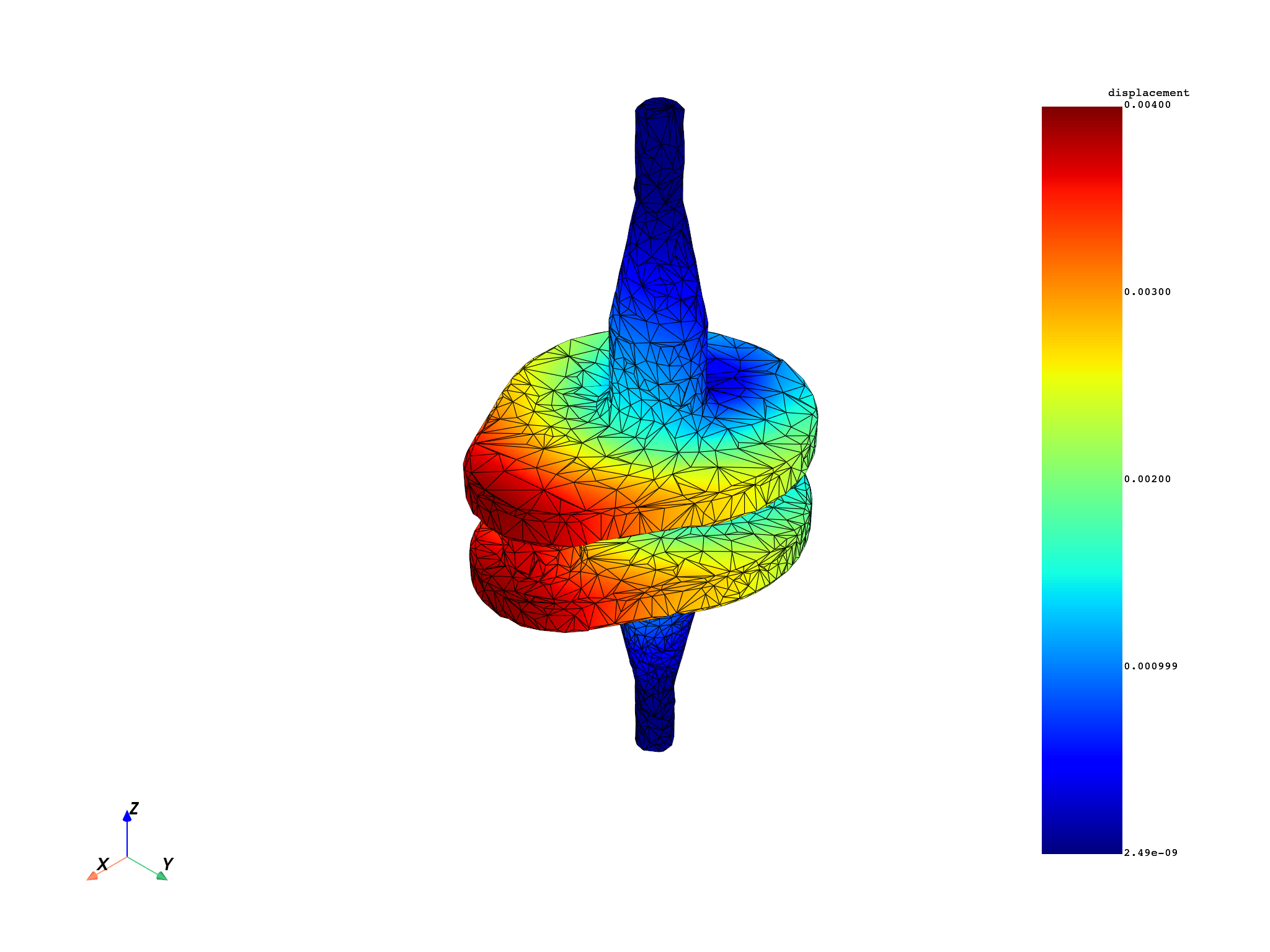
Source field:  69762 entities (solid nodes)
Mapped field:  2471 entities (surface nodes)

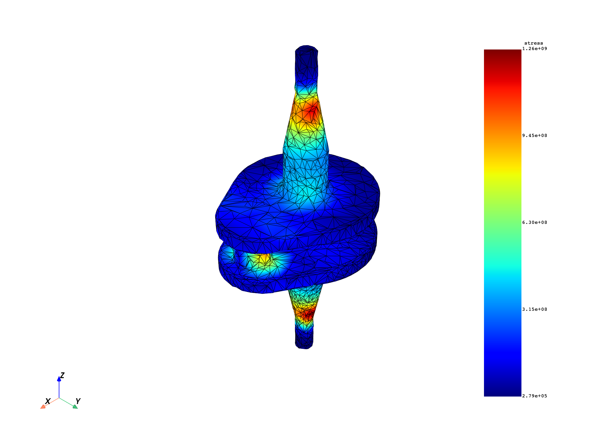
Reuse the workflow for a different result type

The same workflow can be reconnected to map another field type without rebuilding the RBF setup.

stress_fc = model.results.stress.on_location(dpf.locations.nodal).eval()
stress_field = stress_fc[0]

mapping_workflow.connect(pin_name=input_pin_name, inpt=stress_field)
mapped_stress_field = mapping_workflow.get_output(
    pin_name=output_pin_name,
    output_type=dpf.types.field,
)
output_mesh.plot(
    field_or_fields_container=mapped_stress_field, title="Mapped stress on decimated surface"
)

(None, <pyvista.plotting.plotter.Plotter object at 0x00000215A54969D0>)

Add the influence box parameter

The influence box further limits the RBF search window and can improve performance for sparse or asymmetric meshes.

influence_box = 0.01

prepare_op_with_box = ops.mapping.prepare_mapping_workflow(
    input_support=input_mesh,
    output_support=output_mesh,
    filter_radius=filter_radius,
    influence_box=influence_box,
)
mapping_workflow_with_box = prepare_op_with_box.eval()
mapping_workflow_with_box.progress_bar = False
mapping_workflow_with_box.connect(pin_name=input_pin_name, inpt=displacement_field)
mapped_disp_with_box = mapping_workflow_with_box.get_output(
    pin_name=output_pin_name, output_type=dpf.types.field
)
output_mesh.plot(
    field_or_fields_container=mapped_disp_with_box,
    title="Mapped displacement with influence box (decimated surface)",
)

(None, <pyvista.plotting.plotter.Plotter object at 0x00000215A543F3D0>)

Effect of filter radius on mapping quality

A larger filter radius produces smoother interpolation but may lose fine details. Compare the displacement range across several radii.

A reference value is first obtained by running the mapping without setting filter_radius, so the operator uses its built-in default. The swept values are then plotted against this untuned baseline.

ref_prep_op = ops.mapping.prepare_mapping_workflow(
    input_support=input_mesh,
    output_support=output_mesh,
)
ref_workflow: dpf.Workflow = ref_prep_op.eval()
ref_workflow.progress_bar = False
ref_workflow.connect(pin_name=input_pin_name, inpt=displacement_field)
ref_result = ref_workflow.get_output(pin_name=output_pin_name, output_type=dpf.types.field)

filter_radii = [0.001, 0.003, 0.006, 0.01, 0.02, 0.03, 0.04, 0.05]

mean_mags = []
min_mags = []
max_mags = []
for radius in filter_radii:
    prep_op = ops.mapping.prepare_mapping_workflow(
        input_support=input_mesh,
        output_support=output_mesh,
        filter_radius=radius,
    )
    workflow: dpf.Workflow = prep_op.eval()
    workflow.connect(pin_name=input_pin_name, inpt=displacement_field)
    workflow.progress_bar = False
    result = workflow.get_output(pin_name=output_pin_name, output_type=dpf.types.field)
    norm_field = ops.math.norm(field=result).outputs.field()
    min_max_op = ops.min_max.min_max(field=norm_field)
    min_mags.append(min_max_op.outputs.field_min().data[0])
    max_mags.append(min_max_op.outputs.field_max().data[0])
    mean_mags.append(
        ops.math.accumulate(fieldA=norm_field).outputs.field().data[0] / norm_field.scoping.size
    )

ref_norm_field = ops.math.norm(field=ref_result).outputs.field()
ref_min_max_op = ops.min_max.min_max(field=ref_norm_field)
ref_min_mag = ref_min_max_op.outputs.field_min().data[0]
ref_max_mag = ref_min_max_op.outputs.field_max().data[0]
reference_mean_mag = (
    ops.math.accumulate(fieldA=ref_norm_field).outputs.field().data[0] / ref_norm_field.scoping.size
)
print(f"Reference mean displacement magnitude (no filter_radius set): {reference_mean_mag:.4e} m")

fig, ax = plt.subplots()
ax.fill_between(filter_radii, min_mags, max_mags, alpha=0.2, label="Min-max range")
ax.plot(filter_radii, mean_mags, "o-", label="Mean magnitude")
ax.plot(filter_radii, min_mags, "v--", color="tab:blue", alpha=0.6, label="Min magnitude")
ax.plot(filter_radii, max_mags, "^--", color="tab:blue", alpha=0.6, label="Max magnitude")
ax.axhline(
    reference_mean_mag,
    color="gray",
    linestyle="-",
    label=f"Default - mean ({reference_mean_mag:.2e} m)",
)
ax.axhline(ref_min_mag, color="gray", linestyle=":", label=f"Default - min ({ref_min_mag:.2e} m)")
ax.axhline(ref_max_mag, color="gray", linestyle=":", label=f"Default - max ({ref_max_mag:.2e} m)")
ax.set_xlabel("Filter radius (m)")
ax.set_ylabel("Displacement magnitude (m)")
ax.set_title(
    "Effect of filter radius on mapped displacement\n(narrowing min-max band = loss of fine detail)"
)
ax.legend(fontsize="small")
plt.tight_layout()
plt.show()

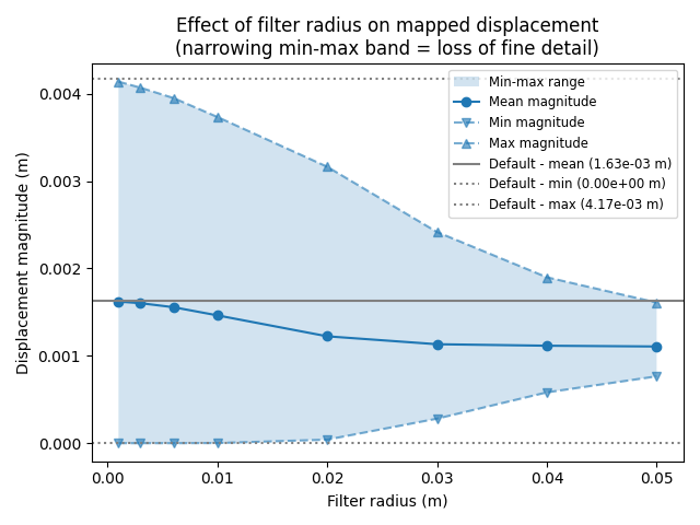
Reference mean displacement magnitude (no filter_radius set): 1.6280e-03 m