Reduced coordinates mapping

Perform high-precision interpolation using a two-step element-local coordinate approach.

This tutorial demonstrates the find_reduced_coordinates / on_reduced_coordinates workflow for mapping field values. In the first step, find_reduced_coordinates locates which element contains each target point and computes the element-local (reference) coordinates. In the second step, on_reduced_coordinates uses those element-local coordinates to perform the interpolation.

Compared to direct Interpolation at coordinates mapping, this approach gives explicit access to element-local positions, enables efficient reuse for multiple field types, and supports higher-accuracy quadratic element interpolation.

Any target point outside the source mesh returns an empty value.

Import modules and load the model

Import the required modules and load a result file.

# Import the ``ansys.dpf.core`` module
# Import NumPy for coordinate manipulation
import matplotlib.pyplot as plt
import numpy as np

from ansys.dpf import core as dpf

# Import the examples and operators modules
from ansys.dpf.core import examples, operators as ops
from ansys.dpf.core.geometry import Line
from ansys.dpf.core.plotter import DpfPlotter

Load model

Download the crankshaft result file and create a Model object.

result_file = examples.download_crankshaft()
model = dpf.Model(data_sources=result_file)
print(model)

DPF Model
------------------------------
Static analysis
Unit system: MKS: m, kg, N, s, V, A, degC
Physics Type: Mechanical
Available results:
     -  node_orientations: Nodal Node Euler Angles
     -  displacement: Nodal Displacement
     -  velocity: Nodal Velocity
     -  acceleration: Nodal Acceleration
     -  reaction_force: Nodal Force
     -  stress: ElementalNodal Stress
     -  elemental_volume: Elemental Volume
     -  stiffness_matrix_energy: Elemental Energy-stiffness matrix
     -  artificial_hourglass_energy: Elemental Hourglass Energy
     -  kinetic_energy: Elemental Kinetic Energy
     -  co_energy: Elemental co-energy
     -  incremental_energy: Elemental incremental energy
     -  thermal_dissipation_energy: Elemental thermal dissipation energy
     -  elastic_strain: ElementalNodal Strain
     -  elastic_strain_eqv: ElementalNodal Strain eqv
     -  element_orientations: ElementalNodal Element Euler Angles
     -  structural_temperature: ElementalNodal Structural temperature
------------------------------
DPF  Meshed Region:
  69762 nodes
  39315 elements
  Unit: m
  With solid (3D) elements
------------------------------
DPF  Time/Freq Support:
  Number of sets: 3
Cumulative     Time (s)       LoadStep       Substep
1              1.000000       1              1
2              2.000000       1              2
3              3.000000       1              3

Extract the mesh

The mesh is needed by both find_reduced_coordinates and on_reduced_coordinates. Use bounding_box to confirm the spatial extent of the model before choosing probe points.

mesh = model.metadata.meshed_region
bb_data = mesh.bounding_box.data[0]  # [xmin, ymin, zmin, xmax, ymax, zmax]
print(
    f"Bounding box: x=[{bb_data[0]:.4f}, {bb_data[3]:.4f}] "
    f"y=[{bb_data[1]:.4f}, {bb_data[4]:.4f}] "
    f"z=[{bb_data[2]:.4f}, {bb_data[5]:.4f}] m"
)

Bounding box: x=[-0.0250, 0.0350] y=[-0.0250, 0.0250] z=[-0.0720, 0.0500] m

Define target coordinates

Create a Field that holds the probe points at which field values should be interpolated.

A line of 8 equally-spaced points is built along the crankshaft z-axis. The range deliberately extends 10 mm beyond each end of the bounding box so that the first and last points fall outside the model—demonstrating how the reduced-coordinates workflow handles coordinates with no containing element.

n_pts = 50
z_pts = np.linspace(bb_data[2] - 0.01, bb_data[5] + 0.01, n_pts)
points = np.column_stack(
    [np.full(n_pts, 0.005), np.zeros(n_pts), z_pts]  # fixed x=5 mm, y=0
)
coords_field = dpf.fields_factory.field_from_array(arr=points)
print(
    f"Probe line: {n_pts} points, z from {z_pts[0]:.4f} to {z_pts[-1]:.4f} m "
    f"(bbox: [{bb_data[2]:.4f}, {bb_data[5]:.4f}])"
)

Probe line: 50 points, z from -0.0820 to 0.0600 m (bbox: [-0.0720, 0.0500])

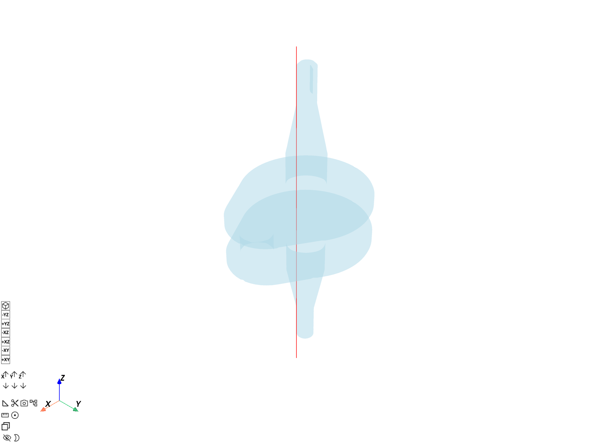
Visualize probe line on the crankshaft

Build a Line from the two endpoints of the probe path and overlay it on a transparent crankshaft mesh.

probe_line = Line([points[0], points[-1]], n_points=n_pts)

pl = DpfPlotter()
pl.add_mesh(probe_line.mesh, color="red", line_width=4)
pl.add_mesh(mesh, style="surface", show_edges=False, opacity=0.3)
pl.show_figure(show_axes=True)

([], <pyvista.plotting.plotter.Plotter object at 0x00000215DA47C210>)

Step 1: Find reduced coordinates and element IDs

Use find_reduced_coordinates to determine which element contains each target point and the corresponding element-local (reference) coordinates.

find_op = ops.mapping.find_reduced_coordinates(
    coordinates=coords_field,
    mesh=mesh,
)
reduced_coords_fc = find_op.outputs.reduced_coordinates()
element_ids_sc = find_op.outputs.element_ids()

print("Reduced coordinates:")
print(reduced_coords_fc)
print("Element IDs:")
print(element_ids_sc)

# The scoping of the reduced-coordinates field records which input probe
# points were found inside an element; the rest fall outside the mesh.
found_ids = reduced_coords_fc[0].scoping.ids  # 1-based input-point indices
in_mesh = np.zeros(n_pts, dtype=bool)
for eid in found_ids:
    in_mesh[eid - 1] = True
print(f"{in_mesh.sum()} of {n_pts} probe points are inside the mesh")
x = z_pts  # use z-coordinate as the x-axis

Reduced coordinates:
DPF  Fields Container
  with 1 field(s)
  defined on labels: Unknown

  with:
  - field 0 {Unknown:  1} with Nodal location, 3 components and 24 entities.

Element IDs:
DPF  Scopings Container
  with 1 scoping(s)
  defined on labels: Unknown

  with:
  - scoping 0 {Unknown:  1, } located on Elemental 24 entities.

24 of 50 probe points are inside the mesh

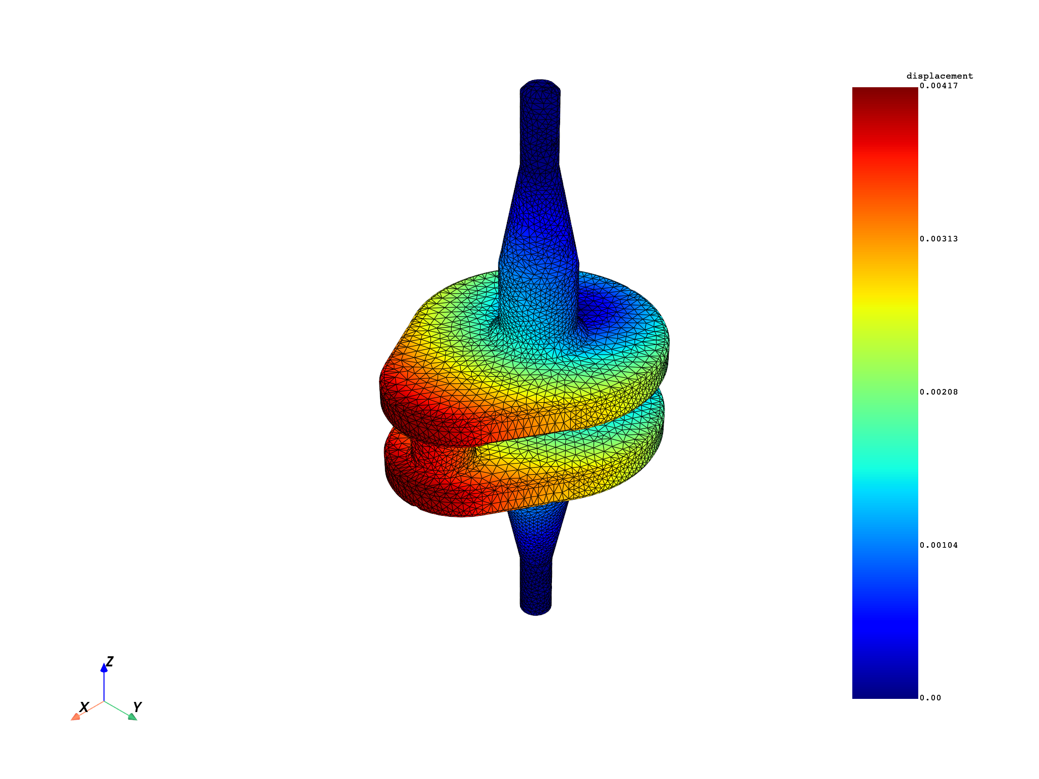
Step 2: Map displacement to reduced coordinates

Use on_reduced_coordinates to interpolate displacement values at the reduced coordinates found in step 1.

displacement_fc = model.results.displacement.eval()
mesh.plot(field_or_fields_container=displacement_fc, title="Crankshaft displacement")

mapping_op = ops.mapping.on_reduced_coordinates(
    fields_container=displacement_fc,
    reduced_coordinates=reduced_coords_fc,
    element_ids=element_ids_sc,
    mesh=mesh,
)
mapped_displacement_fc = mapping_op.eval()

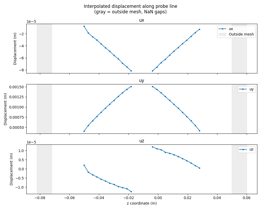
Access mapped results

Extract and display the interpolated displacement values.

mapped_field = mapped_displacement_fc[0]
mapped_data = mapped_field.data
element_ids = element_ids_sc[0]

# Build full arrays (NaN for outside-mesh points)
full_disp = np.full((n_pts, 3), np.nan)
for k, eid in enumerate(mapped_field.scoping.ids):
    full_disp[eid - 1] = mapped_data[k]

# Line plot: displacement components along the probe line.
# Gaps appear where probe points fall outside the mesh.
components = ["ux", "uy", "uz"]

fig, axes = plt.subplots(3, 1, figsize=(10, 8), sharex=True)
for j, (ax, comp) in enumerate(zip(axes, components)):
    y_vals = np.where(in_mesh, full_disp[:, j], np.nan)
    ax.plot(x, y_vals, "o-", ms=3, label=comp)
    ax.axvspan(
        x[0], bb_data[2], color="lightgray", alpha=0.4, label="Outside mesh" if j == 0 else ""
    )
    ax.axvspan(bb_data[5], x[-1], color="lightgray", alpha=0.4)
    ax.set_ylabel("Displacement (m)")
    ax.set_title(comp)
    ax.legend(loc="upper right")
axes[-1].set_xlabel("z coordinate (m)")
plt.suptitle("Interpolated displacement along probe line\n(gray = outside mesh, NaN gaps)")
plt.tight_layout()
plt.show()

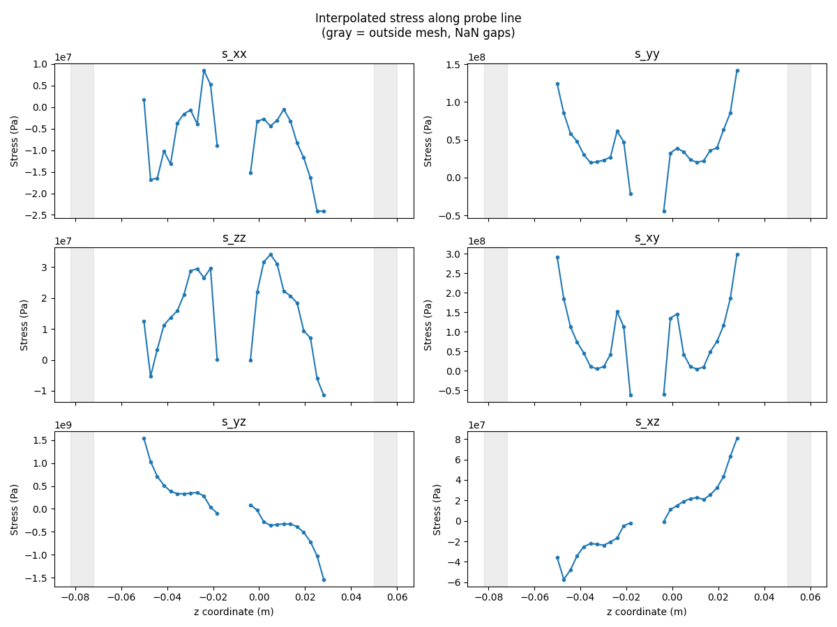
Reuse reduced coordinates for stress

Once the reduced coordinates and element IDs are available they can be reused to map additional result types efficiently without repeating the search step.

stress_fc = model.results.stress.eval()
mapped_stress_fc = ops.mapping.on_reduced_coordinates(
    fields_container=stress_fc,
    reduced_coordinates=reduced_coords_fc,
    element_ids=element_ids_sc,
    mesh=mesh,
).eval()
stress_data_out = mapped_stress_fc[0].data
full_stress = np.full((n_pts, 6), np.nan)
for k, eid in enumerate(mapped_stress_fc[0].scoping.ids):
    full_stress[eid - 1] = stress_data_out[k]

# Line plot: stress components along the probe line.
comp_names = ["s_xx", "s_yy", "s_zz", "s_xy", "s_yz", "s_xz"]

fig, axes = plt.subplots(3, 2, figsize=(12, 9), sharex=True)
for j, (ax, comp) in enumerate(zip(axes.flat, comp_names)):
    y_vals = np.where(in_mesh, full_stress[:, j], np.nan)
    ax.plot(x, y_vals, "o-", ms=3, label=comp)
    ax.axvspan(x[0], bb_data[2], color="lightgray", alpha=0.4)
    ax.axvspan(bb_data[5], x[-1], color="lightgray", alpha=0.4)
    ax.set_ylabel("Stress (Pa)")
    ax.set_title(comp)
for ax in axes[-1]:
    ax.set_xlabel("z coordinate (m)")
plt.suptitle("Interpolated stress along probe line\n(gray = outside mesh, NaN gaps)")
plt.tight_layout()
plt.show()

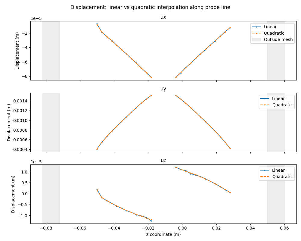
Use quadratic elements for higher precision

For meshes with quadratic elements, enable the use_quadratic_elements option in both operators for higher-order interpolation accuracy.

find_op_quad = ops.mapping.find_reduced_coordinates(
    coordinates=coords_field,
    mesh=mesh,
    use_quadratic_elements=True,
)
reduced_coords_quad_fc = find_op_quad.outputs.reduced_coordinates()
element_ids_quad_sc = find_op_quad.outputs.element_ids()

mapped_disp_quad_fc = ops.mapping.on_reduced_coordinates(
    fields_container=displacement_fc,
    reduced_coordinates=reduced_coords_quad_fc,
    element_ids=element_ids_quad_sc,
    mesh=mesh,
    use_quadratic_elements=True,
).eval()

quad_data_out = mapped_disp_quad_fc[0].data
full_quad = np.full((n_pts, 3), np.nan)
for k, eid in enumerate(mapped_disp_quad_fc[0].scoping.ids):
    full_quad[eid - 1] = quad_data_out[k]

# Line plot comparison: linear vs quadratic interpolation
fig, axes = plt.subplots(3, 1, figsize=(10, 8), sharex=True)
for j, (ax, comp) in enumerate(zip(axes, components)):
    y_lin = np.where(in_mesh, full_disp[:, j], np.nan)
    y_quad = np.where(in_mesh, full_quad[:, j], np.nan)
    ax.plot(x, y_lin, "o-", ms=2, label="Linear")
    ax.plot(x, y_quad, "s--", ms=2, label="Quadratic")
    ax.axvspan(
        x[0], bb_data[2], color="lightgray", alpha=0.4, label="Outside mesh" if j == 0 else ""
    )
    ax.axvspan(bb_data[5], x[-1], color="lightgray", alpha=0.4)
    ax.set_ylabel("Displacement (m)")
    ax.set_title(comp)
    ax.legend(loc="upper right")
axes[-1].set_xlabel("z coordinate (m)")
plt.suptitle("Displacement: linear vs quadratic interpolation along probe line")
plt.tight_layout()
plt.show()