Interpolation at coordinates

Interpolate field values at arbitrary spatial coordinates using element shape functions.

This tutorial demonstrates how to use the on_coordinates operator to extract result values at specific locations in a model. The operator interpolates field values at arbitrary coordinates using the mesh shape functions, enabling you to extract results along paths, at sensor locations, or on custom grids.

Any target point outside the source mesh returns an empty value.

Import modules and load the model

Import the required modules and load a result file.

# Import the ``ansys.dpf.core`` module
# Import NumPy for coordinate manipulation
import matplotlib.pyplot as plt
import numpy as np

from ansys.dpf import core as dpf
from ansys.dpf.core import examples, operators as ops
from ansys.dpf.core.geometry import Line
from ansys.dpf.core.plotter import DpfPlotter

Load model

Download the crankshaft result file and create a Model object.

result_file = examples.download_crankshaft()
model = dpf.Model(data_sources=result_file)
print(model)

DPF Model
------------------------------
Static analysis
Unit system: MKS: m, kg, N, s, V, A, degC
Physics Type: Mechanical
Available results:
     -  node_orientations: Nodal Node Euler Angles
     -  displacement: Nodal Displacement
     -  velocity: Nodal Velocity
     -  acceleration: Nodal Acceleration
     -  reaction_force: Nodal Force
     -  stress: ElementalNodal Stress
     -  elemental_volume: Elemental Volume
     -  stiffness_matrix_energy: Elemental Energy-stiffness matrix
     -  artificial_hourglass_energy: Elemental Hourglass Energy
     -  kinetic_energy: Elemental Kinetic Energy
     -  co_energy: Elemental co-energy
     -  incremental_energy: Elemental incremental energy
     -  thermal_dissipation_energy: Elemental thermal dissipation energy
     -  elastic_strain: ElementalNodal Strain
     -  elastic_strain_eqv: ElementalNodal Strain eqv
     -  element_orientations: ElementalNodal Element Euler Angles
     -  structural_temperature: ElementalNodal Structural temperature
------------------------------
DPF  Meshed Region:
  69762 nodes
  39315 elements
  Unit: m
  With solid (3D) elements
------------------------------
DPF  Time/Freq Support:
  Number of sets: 3
Cumulative     Time (s)       LoadStep       Substep
1              1.000000       1              1
2              2.000000       1              2
3              3.000000       1              3

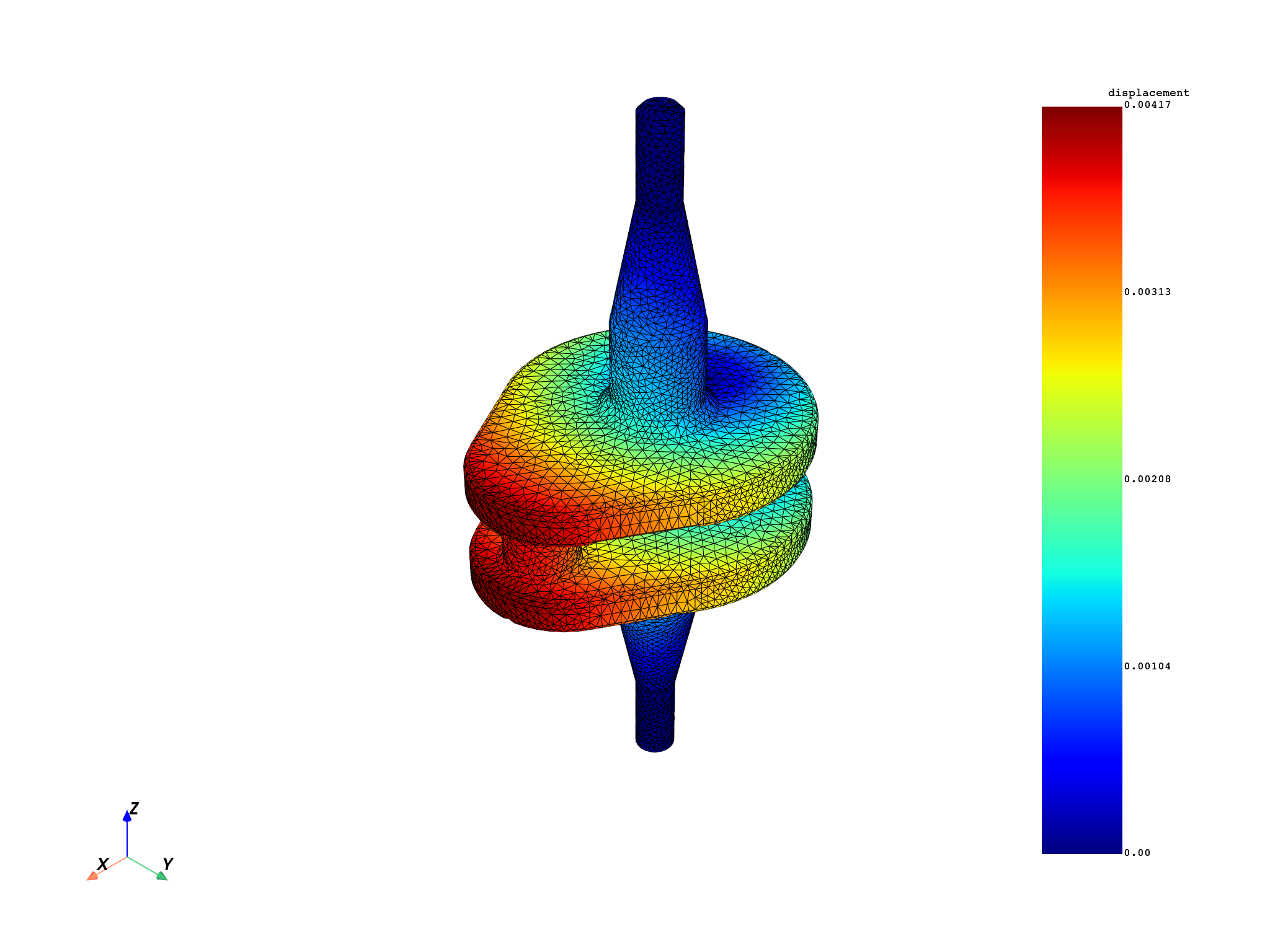
Extract displacement results

Get the displacement results from the model as a FieldsContainer.

displacement_fc = model.results.displacement.eval()
mesh = model.metadata.meshed_region
mesh.plot(field_or_fields_container=displacement_fc, title="Crankshaft displacement")

(None, <pyvista.plotting.plotter.Plotter object at 0x00000215C147C690>)

Define coordinates of interest

Define a line of 8 equally-spaced probe points along the crankshaft z-axis. The range deliberately extends 10 mm beyond each end of the bounding box so that the first and last points fall outside the model—demonstrating how on_coordinates returns an empty value for coordinates with no containing element.

bb_data = mesh.bounding_box.data[0]  # [xmin, ymin, zmin, xmax, ymax, zmax]
print(
    f"Bounding box: x=[{bb_data[0]:.4f}, {bb_data[3]:.4f}] "
    f"y=[{bb_data[1]:.4f}, {bb_data[4]:.4f}] "
    f"z=[{bb_data[2]:.4f}, {bb_data[5]:.4f}] m"
)

n_pts = 50
z_pts = np.linspace(bb_data[2] - 0.01, bb_data[5] + 0.01, n_pts)
points = np.column_stack(
    [np.full(n_pts, 0.005), np.zeros(n_pts), z_pts]  # fixed x=5 mm, y=0
)
coords_field = dpf.fields_factory.field_from_array(arr=points)
print(
    f"Probe line: {n_pts} points, z from {z_pts[0]:.4f} to {z_pts[-1]:.4f} m "
    f"(bbox: [{bb_data[2]:.4f}, {bb_data[5]:.4f}])"
)

Bounding box: x=[-0.0250, 0.0350] y=[-0.0250, 0.0250] z=[-0.0720, 0.0500] m
Probe line: 50 points, z from -0.0820 to 0.0600 m (bbox: [-0.0720, 0.0500])

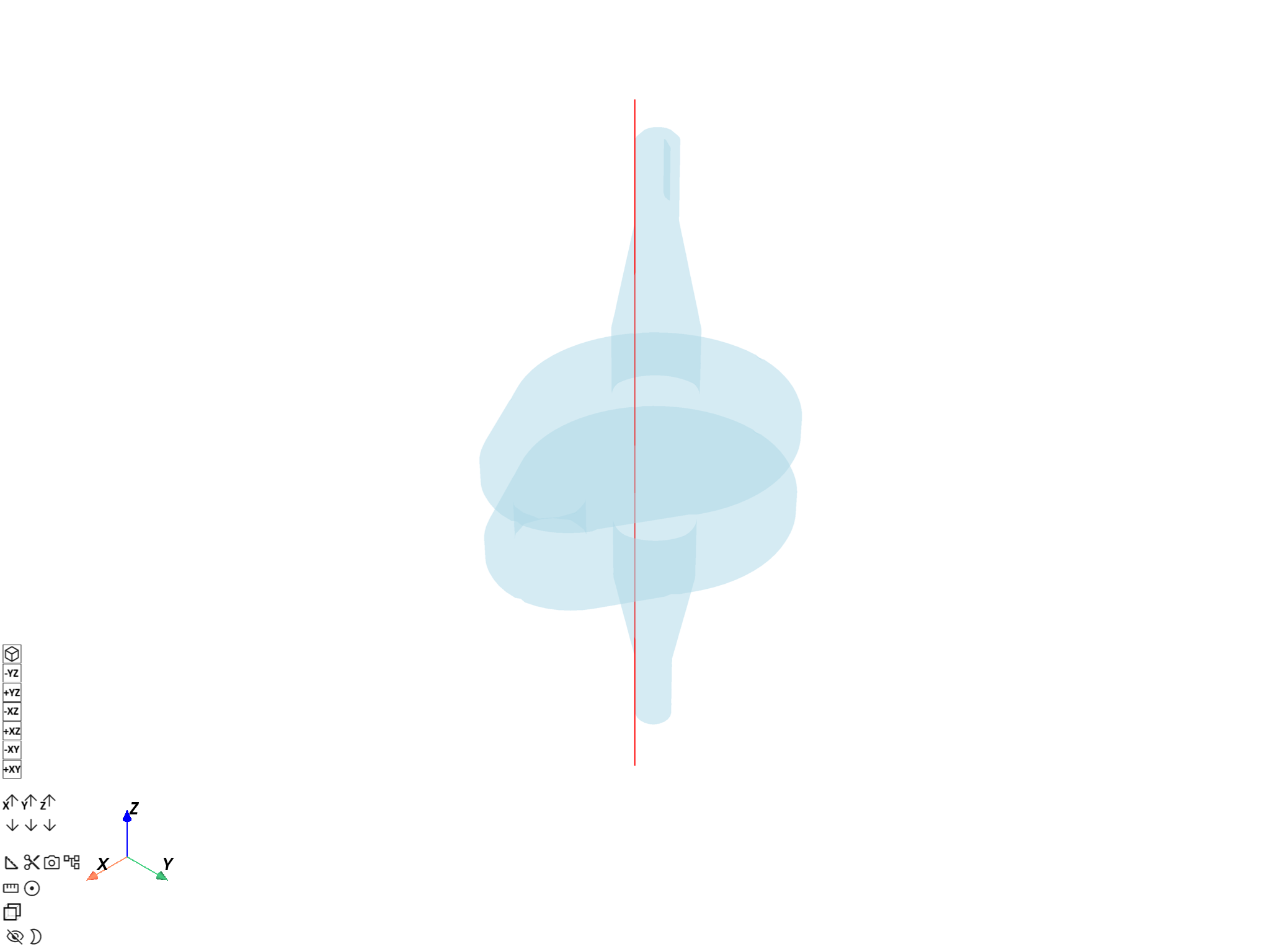
Visualize probe line on the crankshaft

Build a Line from the two endpoints of the probe path and overlay it on a transparent crankshaft mesh so the spatial context is immediately visible.

probe_line = Line([points[0], points[-1]], n_points=n_pts)

pl = DpfPlotter()
pl.add_mesh(probe_line.mesh, color="red", line_width=4)
pl.add_mesh(mesh, style="surface", show_edges=False, opacity=0.3)
pl.show_figure(show_axes=True)

([], <pyvista.plotting.plotter.Plotter object at 0x00000215D1691850>)

Map displacement to coordinates

Use the on_coordinates operator to interpolate displacement values at the defined coordinates.

mapping_op = ops.mapping.on_coordinates(
    fields_container=displacement_fc,
    coordinates=coords_field,
)
mapped_displacement_fc = mapping_op.eval()

Access mapped results

The output field only contains entities for probe points that were found inside an element. Build a full (n_pts, 3) array—filling NaN for coordinates outside the mesh—to keep a one-to-one correspondence with the input probe line.

mapped_field = mapped_displacement_fc[0]
mapped_data = mapped_field.data
found_ids = mapped_field.scoping.ids  # 1-based indices of found probe points

full_disp = np.full((n_pts, 3), np.nan)
for k, eid in enumerate(found_ids):
    full_disp[eid - 1] = mapped_data[k]

in_mesh = ~np.isnan(full_disp[:, 0])
print(f"{in_mesh.sum()} of {n_pts} probe points are inside the mesh")

components = ["ux", "uy", "uz"]
x = z_pts  # use z-coordinate as the x-axis

# Line plot: displacement components along the probe line.
# Gaps appear where probe points fall outside the mesh.
fig, axes = plt.subplots(3, 1, figsize=(10, 8), sharex=True)
for j, (ax, comp) in enumerate(zip(axes, components)):
    y_vals = np.where(in_mesh, full_disp[:, j], np.nan)
    ax.plot(x, y_vals, "o-", ms=3, label=comp)
    ax.axvspan(
        x[0], bb_data[2], color="lightgray", alpha=0.4, label="Outside mesh" if j == 0 else ""
    )
    ax.axvspan(bb_data[5], x[-1], color="lightgray", alpha=0.4)
    ax.set_ylabel("Displacement (m)")
    ax.set_title(comp)
    ax.legend(loc="upper right")
axes[-1].set_xlabel("z coordinate (m)")
plt.suptitle("Interpolated displacement along probe line\n(gray = outside mesh, NaN gaps)")
plt.tight_layout()
plt.show()

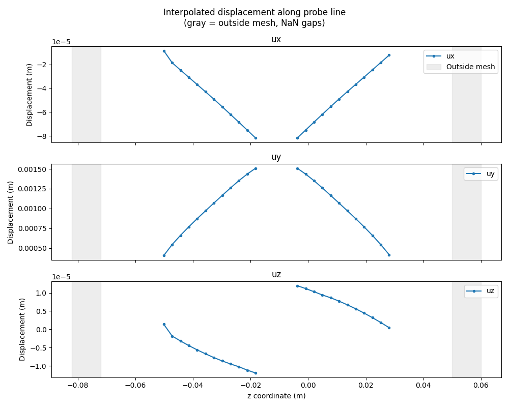
24 of 50 probe points are inside the mesh

Provide mesh explicitly

If the input fields do not have a mesh in their support, you can provide the mesh explicitly via the mesh pin.

mapping_op_with_mesh = ops.mapping.on_coordinates(
    fields_container=displacement_fc,
    coordinates=coords_field,
    mesh=mesh,
)
mapped_displacement_with_mesh = mapping_op_with_mesh.eval()

Adjust tolerance for coordinate search

Control the tolerance used in the iterative algorithm that locates coordinates inside the mesh. The default value is 5e-5.

mapping_op_with_tol = ops.mapping.on_coordinates(
    fields_container=displacement_fc,
    coordinates=coords_field,
    tolerance=1e-4,
)
mapped_displacement_with_tol = mapping_op_with_tol.eval()

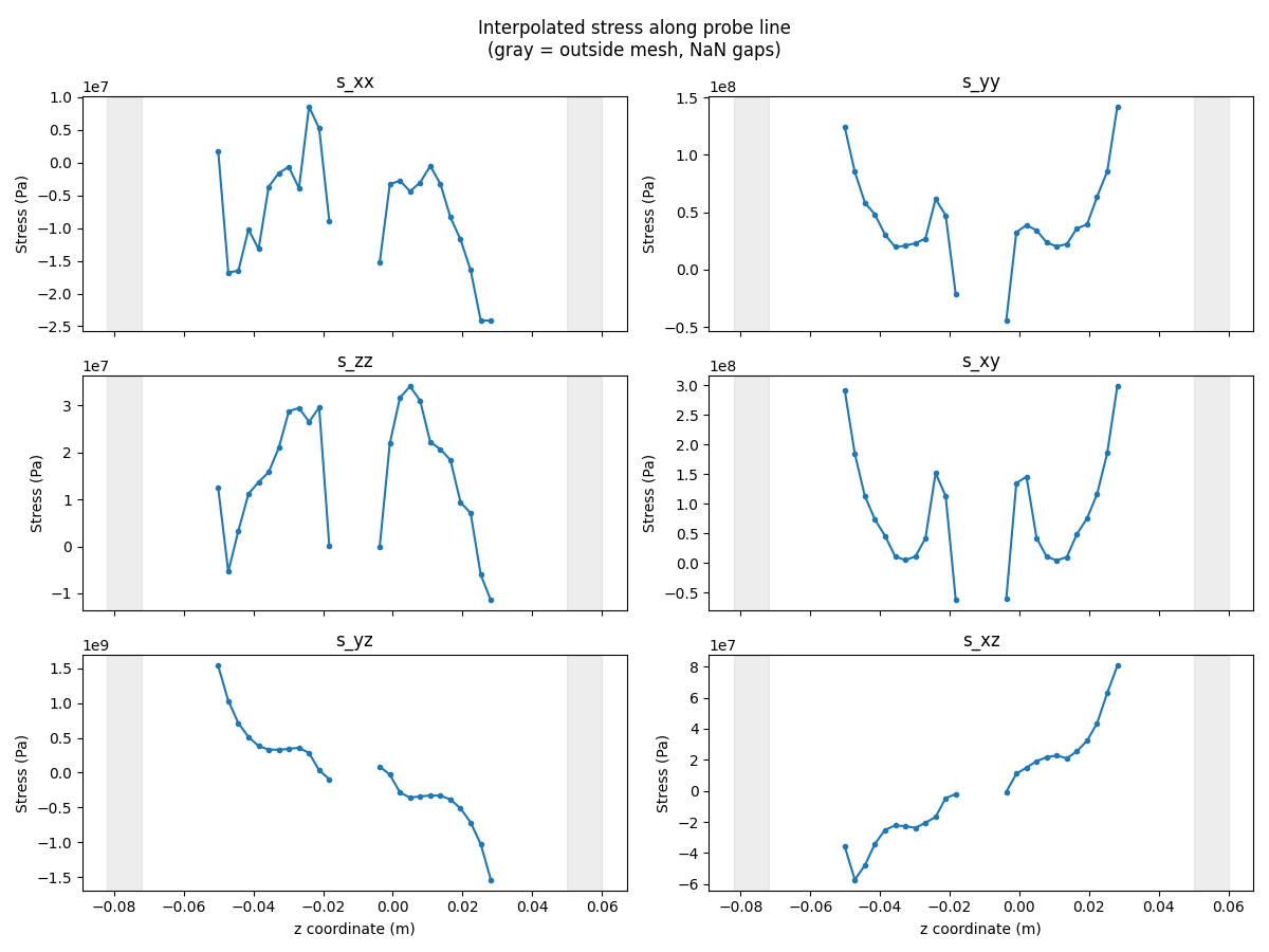
Map multiple result types

The same coordinates can be reused to map different result types.

stress_fc = model.results.stress.eval()
mapped_stress_fc = ops.mapping.on_coordinates(
    fields_container=stress_fc,
    coordinates=coords_field,
).eval()

stress_data_out = mapped_stress_fc[0].data
found_stress_ids = mapped_stress_fc[0].scoping.ids
full_stress = np.full((n_pts, 6), np.nan)
for k, eid in enumerate(found_stress_ids):
    full_stress[eid - 1] = stress_data_out[k]

comp_names = ["s_xx", "s_yy", "s_zz", "s_xy", "s_yz", "s_xz"]

fig, axes = plt.subplots(3, 2, figsize=(12, 9), sharex=True)
for j, (ax, comp) in enumerate(zip(axes.flat, comp_names)):
    y_vals = np.where(in_mesh, full_stress[:, j], np.nan)
    ax.plot(x, y_vals, "o-", ms=3, label=comp)
    ax.axvspan(x[0], bb_data[2], color="lightgray", alpha=0.4)
    ax.axvspan(bb_data[5], x[-1], color="lightgray", alpha=0.4)
    ax.set_ylabel("Stress (Pa)")
    ax.set_title(comp)
for ax in axes[-1]:
    ax.set_xlabel("z coordinate (m)")
plt.suptitle("Interpolated stress along probe line\n(gray = outside mesh, NaN gaps)")
plt.tight_layout()
plt.show()