Compute and plot 2D streamlines

This example shows you how to compute and plot streamlines of fluid simulation results, for 2D models.

Note

This example requires DPF 7.0 (ansys-dpf-server-2024-1-pre0) or above. For more information, see Compatibility.

Plot surface streamlines

Import modules, create the data sources and the model

Import modules:

from ansys.dpf import core as dpf
from ansys.dpf.core import examples
from ansys.dpf.core.helpers.streamlines import compute_streamlines
from ansys.dpf.core.plotter import DpfPlotter

Create data sources for fluids simulation result:

fluent_files = examples.download_fluent_multi_species()
ds_fluent = dpf.DataSources()
ds_fluent.set_result_file_path(fluent_files["cas"], "cas")
ds_fluent.add_file_path(fluent_files["dat"], "dat")

Create model from fluid simulation result data sources:

m_fluent = dpf.Model(ds_fluent)

Get meshed region and velocity data

Meshed region is used as the geometric base to compute the streamlines. Velocity data is used to compute the streamlines. The velocity data must be nodal.

Get the meshed region:

meshed_region = m_fluent.metadata.meshed_region

Get the velocity result at nodes:

velocity_op = m_fluent.results.velocity()
fc = velocity_op.outputs.fields_container()
field = dpf.operators.averaging.to_nodal_fc(fields_container=fc).outputs.fields_container()[0]

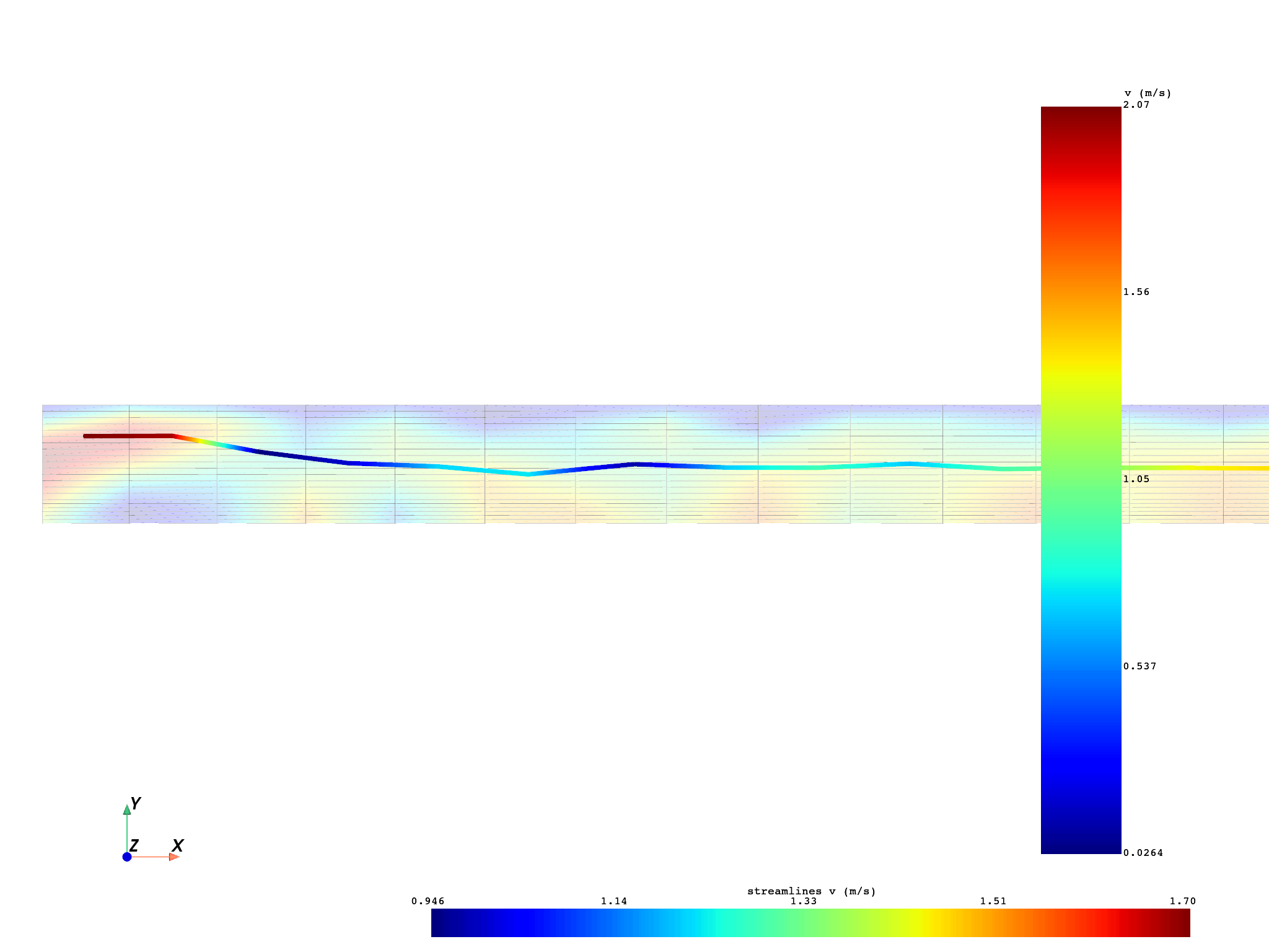
Compute single streamline

single_2d_streamline, single_2d_source = compute_streamlines(
    meshed_region=meshed_region,
    field=field,
    start_position=(0.005, 0.0005, 0.0),
    surface_streamlines=True,
    return_source=True,
)

Plot single streamline

pl_single = DpfPlotter()
pl_single.add_field(field, meshed_region, opacity=0.2)
pl_single.add_streamlines(
    streamlines=single_2d_streamline,
    source=single_2d_source,
    radius=0.00002,
)
# Use the PyVista 'cpos' optional argument to control the camera position.
# To easily save a camera position, plot the figure a first time with the argument
# 'return_cpos=True'. This will make the ``DpfPlotter.show_figure`` function return
# the camera position at the time the PyVista interactive plotting window is closed.
# You can also define a plane to use for the camera with 'cpos="xy"'.
# In this case the camera will fit the entire model in the window.
# Starting from a returned 'cpos', you can build a custom camera position, such as:
cpos = [
    (0.005, 0.0004, 0.015),  # Camera position (X, Y, Z)
    (0.005, 0.0004, 0.0),  # Target point (X, Y, Z)
    (0.0, 1.0, 0.0),  # Upward direction (+y)
]
return_cpos = pl_single.show_figure(return_cpos=True, cpos=cpos, show_axes=True)
print(return_cpos)

[(0.005, 0.0004, 0.015),
 (0.005, 0.0004, 0.0),
 (0.0, 1.0, 0.0)]

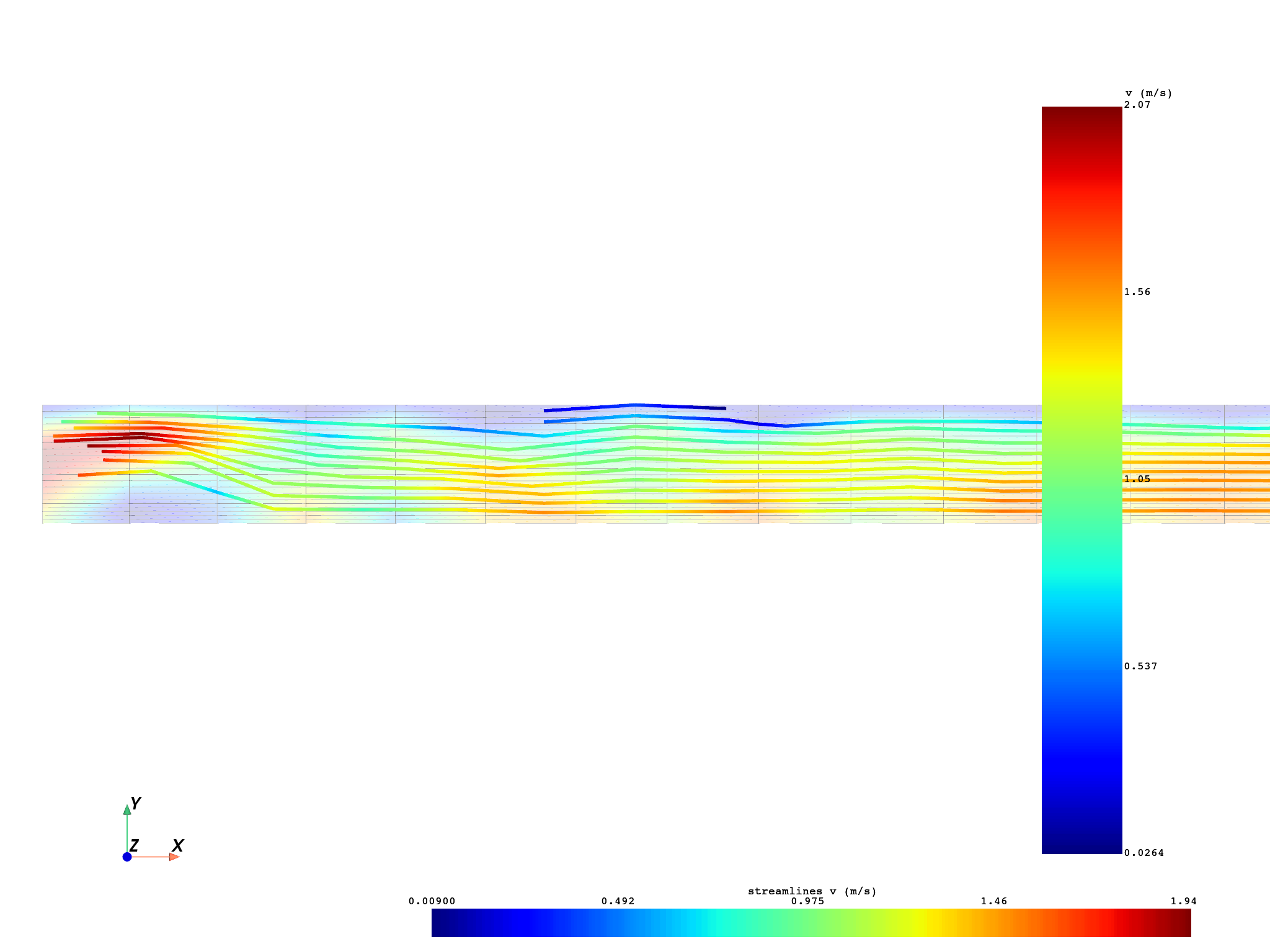
Compute multiple streamlines

multiple_2d_streamlines, multiple_2d_source = compute_streamlines(
    meshed_region=meshed_region,
    field=field,
    pointa=(0.005, 0.0001, 0.0),
    pointb=(0.005, 0.001, 0.0),
    n_points=10,
    surface_streamlines=True,
    return_source=True,
)

Plot multiple streamlines

pl_multiple = DpfPlotter()
pl_multiple.add_field(field, meshed_region, opacity=0.2)
pl_multiple.add_streamlines(
    streamlines=multiple_2d_streamlines,
    source=multiple_2d_source,
    radius=0.000015,
)
pl_multiple.show_figure(cpos=cpos, show_axes=True)