Compute and plot 3D streamlines

This example shows you how to compute and plot streamlines of fluid simulation results, for 3D models.

Note

This example requires DPF 7.0 (ansys-dpf-server-2024-1-pre0) or above. For more information, see Compatibility.

Compute and plot streamlines from single source

Import modules, create the data sources and the model

Import modules:

from ansys.dpf import core as dpf
from ansys.dpf.core import examples
from ansys.dpf.core.helpers.streamlines import compute_streamlines
from ansys.dpf.core.plotter import DpfPlotter

Create data sources for fluids simulation result:

fluent_files = examples.download_fluent_mixing_elbow_steady_state()
ds_fluent = dpf.DataSources()
ds_fluent.set_result_file_path(fluent_files["cas"][0], "cas")
ds_fluent.add_file_path(fluent_files["dat"][1], "dat")

Create model from fluid simulation result data sources:

m_fluent = dpf.Model(ds_fluent)

Get meshed region and velocity data

Meshed region is used as geometric base to compute the streamlines. Velocity data is used to compute the streamlines. The velocity data must be nodal.

Get the meshed region:

meshed_region = m_fluent.metadata.meshed_region

Get the velocity result at nodes:

velocity_op = m_fluent.results.velocity()
fc = velocity_op.outputs.fields_container()
field = dpf.operators.averaging.to_nodal_fc(fields_container=fc).outputs.fields_container()[0]

Compute and plot the streamlines adjusting the request

The following steps show you how to create streamlines using DpfPlotter, with several sets of parameters. It demonstrates the issues that can happen and the adjustments that you can make.

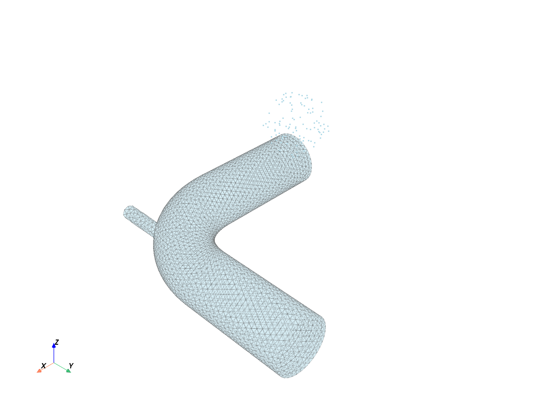
First, Streamlines and StreamlinesSource objects are created. The StreamlinesSource is available using the ‘return_source’ argument. Then, you can correctly set the source coordinates using the “source_center” argument that moves the source center, and “permissive” option that allows you to display the source even, if the computed streamline size is zero. Default value for “permissive” argument is True. If permissive is set to False, the “add_streamlines” method throws.

streamline_obj, source_obj = compute_streamlines(
    meshed_region=meshed_region,
    field=field,
    return_source=True,
    source_center=(0.1, 0.1, 0.2),
)
pl1 = DpfPlotter()
pl1.add_mesh(meshed_region=meshed_region, opacity=0.3)
pl1.add_streamlines(
    streamlines=streamline_obj,
    source=source_obj,
    permissive=True,
)
pl1.show_figure(show_axes=True)

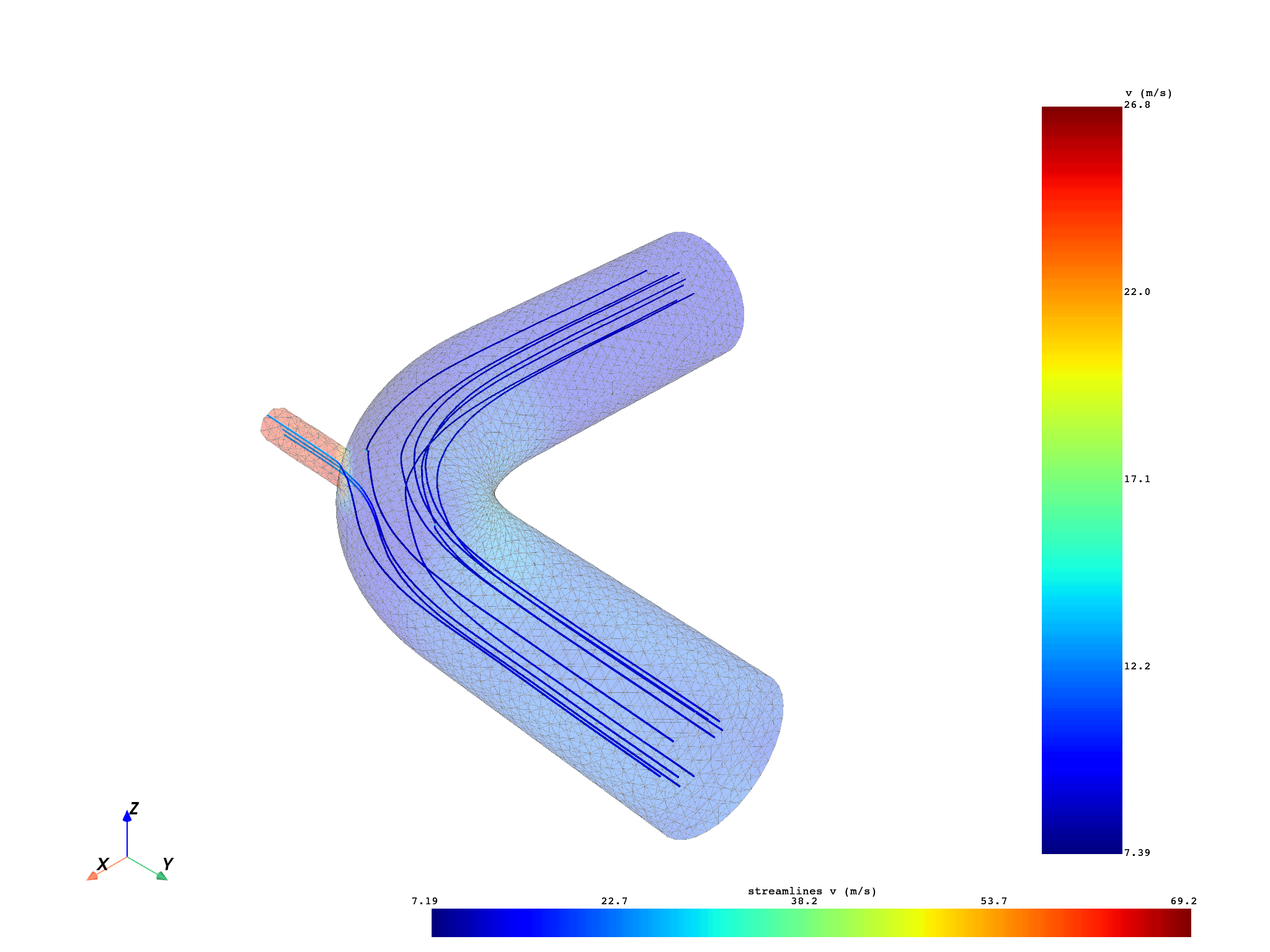
After the adjustment, the correct values for the “source_center” argument are set. You can remove the “permissive” option. You can display velocity data with a small opacity value to avoid hiding the streamlines. More settings are added to adapt the streamlines creation to the geometry and the data of the model: - radius: streamlines radius - n_points: source number of points - source_radius - max_time: maximum integration time of the streamline. It controls the streamline length.

streamline_obj, source_obj = compute_streamlines(
    meshed_region=meshed_region,
    field=field,
    return_source=True,
    source_center=(0.56, 0.48, 0.0),
    n_points=10,
    source_radius=0.075,
    max_time=10.0,
)
pl2 = DpfPlotter()
pl2.add_field(field, meshed_region, opacity=0.2)
pl2.add_streamlines(
    streamlines=streamline_obj,
    source=source_obj,
    radius=0.001,
)
pl2.show_figure(show_axes=True)

Compute and plot streamlines from several sources

Get data to plot

Create data sources for fluid simulation result:

files_cfx = examples.download_cfx_heating_coil()
ds_cfx = dpf.DataSources()
ds_cfx.set_result_file_path(files_cfx["cas"], "cas")
ds_cfx.add_file_path(files_cfx["dat"], "dat")

Create model from fluid simulation result data sources:

m_cfx = dpf.Model(ds_cfx)

Get meshed region and velocity data

meshed_region = m_cfx.metadata.meshed_region
velocity_op = m_cfx.results.velocity()
field = velocity_op.outputs.fields_container()[0]

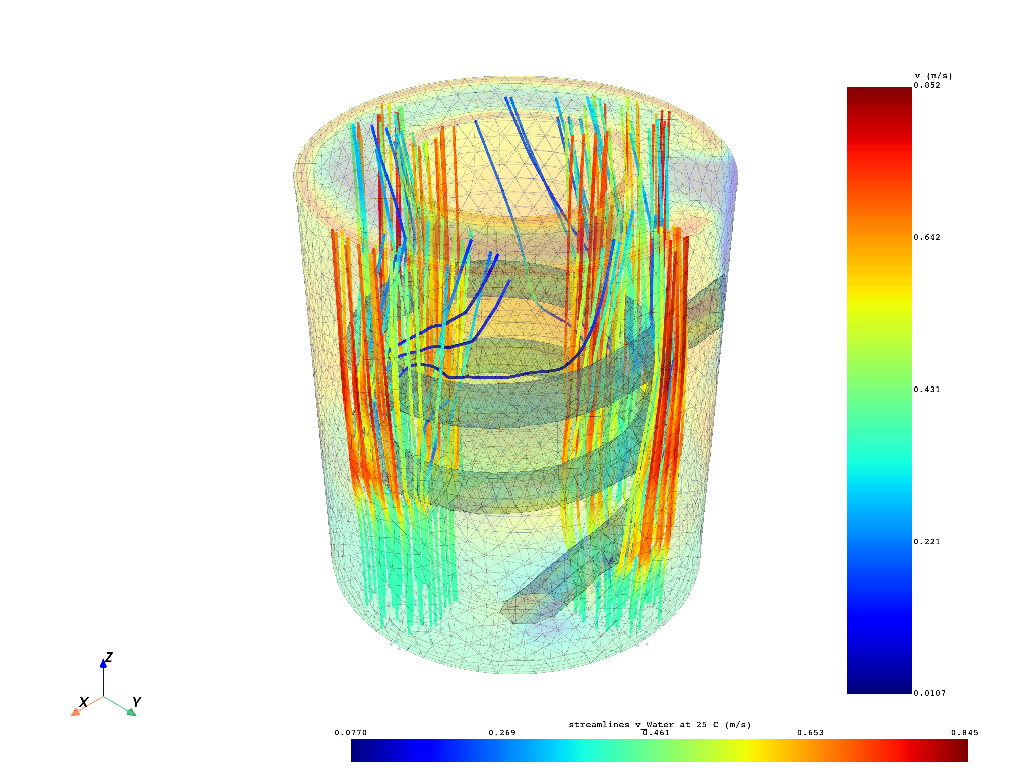
Compute streamlines from different sources

Compute streamlines from different sources:

streamline_1, source_1 = compute_streamlines(
    meshed_region=meshed_region,
    field=field,
    return_source=True,
    source_radius=0.25,
    source_center=(0.75, 0.0, 0.0),
)
streamline_2, source_2 = compute_streamlines(
    meshed_region=meshed_region,
    field=field,
    return_source=True,
    source_radius=0.25,
    source_center=(0.0, 0.75, 0.0),
)
streamline_3, source_3 = compute_streamlines(
    meshed_region=meshed_region,
    field=field,
    return_source=True,
    source_radius=0.25,
    source_center=(-0.75, 0.0, 0.0),
)
streamline_4, source_4 = compute_streamlines(
    meshed_region=meshed_region,
    field=field,
    return_source=True,
    source_radius=0.25,
    source_center=(0.0, -0.75, 0.0),
)

Plot streamlines from different sources

pl = DpfPlotter()
pl.add_field(field, meshed_region, opacity=0.2)
pl.add_streamlines(
    streamlines=streamline_1,
    source=source_1,
    radius=0.007,
)
pl.add_streamlines(
    streamlines=streamline_2,
    source=source_2,
    radius=0.007,
)
pl.add_streamlines(
    streamlines=streamline_3,
    source=source_3,
    radius=0.007,
)
pl.add_streamlines(
    streamlines=streamline_4,
    source=source_4,
    radius=0.007,
)
pl.show_figure(show_axes=True)