Add nodal labels on plots

You can add use label properties to add custom labels to specific nodes. If the label for a node is not defined or None, the nodal scalar value of the currently active field at that node is shown. If no field is active, the node ID is shown.

Import the dpf_core module, included examples files, and the DpfPlotter module.

from ansys.dpf import core as dpf
from ansys.dpf.core import examples
from ansys.dpf.core.plotter import DpfPlotter

Open an example and print the Model object. The Model class helps to organize access methods for the result by keeping track of the operators and data sources used by the result file.

Printing the model displays this metadata:

• Analysis type

• Available results

• Size of the mesh

• Number of results

model = dpf.Model(examples.find_msup_transient())
print(model)

DPF Model
------------------------------
Transient analysis
Unit system: MKS: m, kg, N, s, V, A, degC
Physics Type: Mechanical
Available results:
     -  displacement: Nodal Displacement
     -  velocity: Nodal Velocity
     -  acceleration: Nodal Acceleration
     -  reaction_force: Nodal Force
     -  stress: ElementalNodal Stress
     -  elemental_volume: Elemental Volume
     -  stiffness_matrix_energy: Elemental Energy-stiffness matrix
     -  artificial_hourglass_energy: Elemental Hourglass Energy
     -  thermal_dissipation_energy: Elemental thermal dissipation energy
     -  kinetic_energy: Elemental Kinetic Energy
     -  co_energy: Elemental co-energy
     -  incremental_energy: Elemental incremental energy
     -  elastic_strain: ElementalNodal Strain
------------------------------
DPF  Meshed Region:
  393 nodes
  40 elements
  Unit: m
  With solid (3D) elements
------------------------------
DPF  Time/Freq Support:
  Number of sets: 20
Cumulative     Time (s)       LoadStep       Substep
1              0.010000       1              1
2              0.020000       1              2
3              0.030000       1              3
4              0.040000       1              4
5              0.050000       1              5
6              0.060000       1              6
7              0.070000       1              7
8              0.080000       1              8
9              0.090000       1              9
10             0.100000       1              10
11             0.110000       1              11
12             0.120000       1              12
13             0.130000       1              13
14             0.140000       1              14
15             0.150000       1              15
16             0.160000       1              16
17             0.170000       1              17
18             0.180000       1              18
19             0.190000       1              19
20             0.200000       1              20

Get the meshed region.

mesh_set = model.metadata.meshed_region

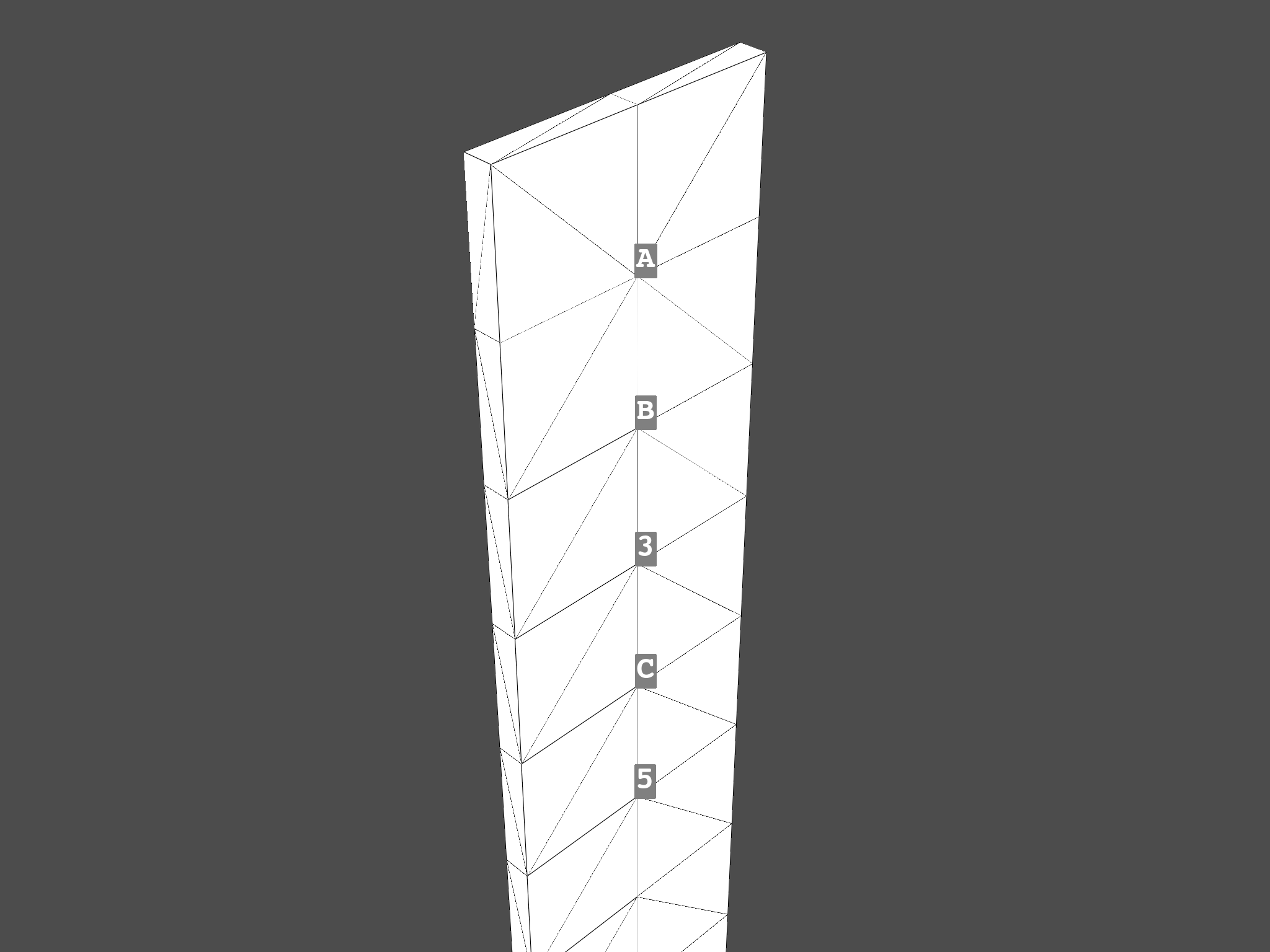
# One can plot the mesh with labels and/or node IDs shown
# for the first five nodes of the mesh.
plot = DpfPlotter()
plot.add_node_labels(
    nodes=mesh_set.nodes.scoping.ids[:5],
    meshed_region=mesh_set,
    labels=["A", "B", None, "C"],
    font_size=50,
)
plot.show_figure(
    cpos=[
        (0.3533494514377904, 0.312496303079723, 1.1859368974825752),
        (-0.07891143256220956, -0.11976458092027707, 0.7536760134825755),
        (0.0, 0.0, 1.0),
    ]
)
# sphinx_gallery_thumbnail_number = 2

Get the stress tensor and connect time scoping. Make sure that you define dpf.locations.nodal as the scoping location because labels are supported only for nodal results.

stress_tensor = model.results.stress()
stress_tensor.inputs.time_scoping([20])
stress_tensor.inputs.requested_location(dpf.locations.nodal)
# field = stress_tensor.outputs.fields_container.get_data()[0]

norm_op = dpf.operators.math.norm_fc()
norm_op.inputs.connect(stress_tensor)
field_norm_stress = norm_op.outputs.fields_container()[0]
print(field_norm_stress)

norm_op2 = dpf.Operator("norm_fc")
disp = model.results.displacement()
disp.inputs.time_scoping.connect([20])
norm_op2.inputs.connect(disp.outputs)
field_norm_disp = norm_op2.outputs.fields_container()[0]
print(field_norm_disp)

DPF stress_0.2s Field
  Location: Nodal
  Unit: Pa
  393 entities
  Data: 1 components and 393 elementary data

  Nodal
  IDs                   data(Pa)
  ------------          ----------
  9                     1.400332e+07

  96                    1.399264e+07

  95                    1.171429e+07

  ...


DPF displacement_0.2s Field
  Location: Nodal
  Unit: m
  393 entities
  Data: 1 components and 393 elementary data

  Nodal
  IDs                   data(m)
  ------------          ----------
  9                     3.106681e-03

  96                    3.101395e-03

  95                    3.714017e-03

  ...

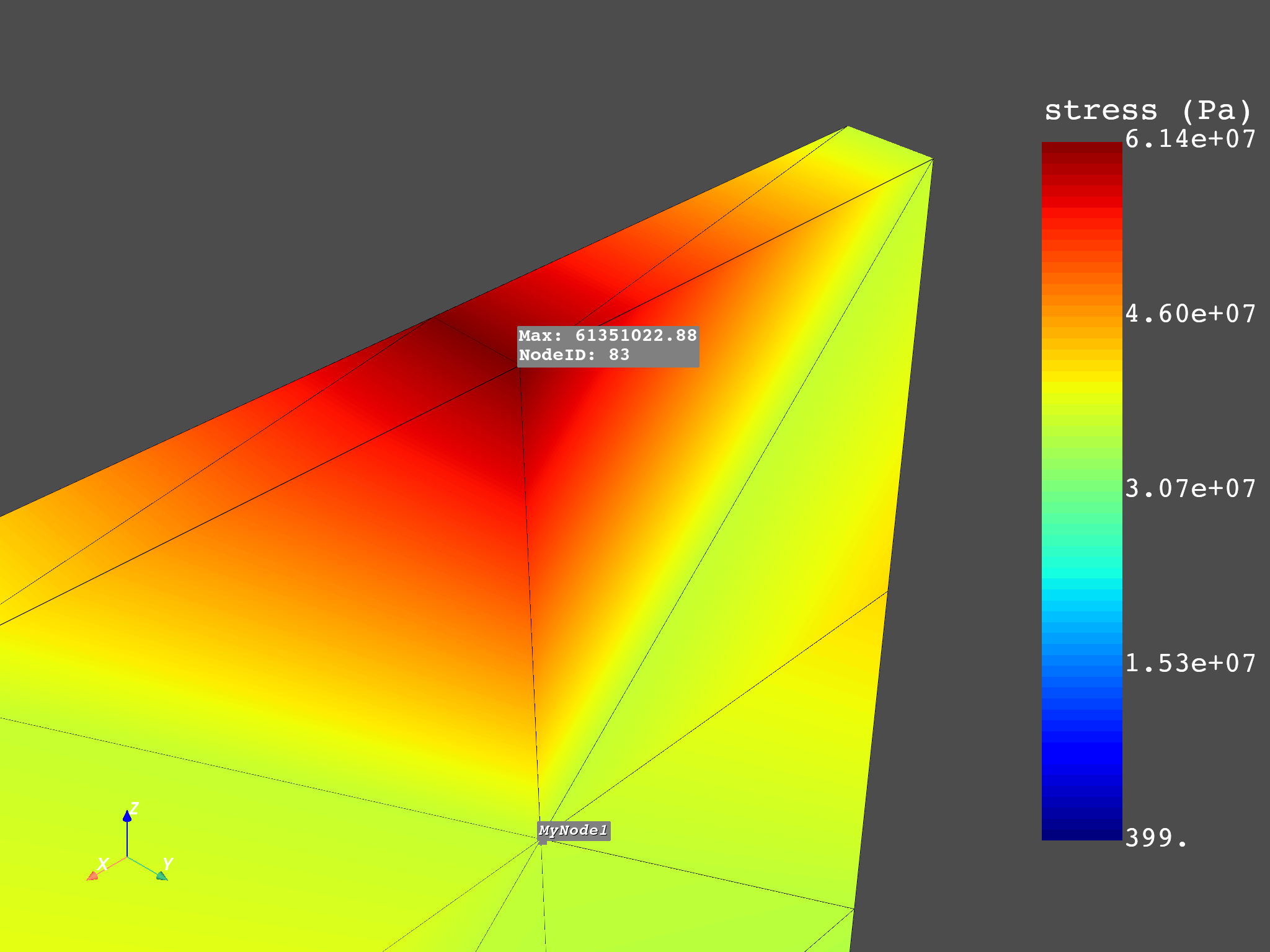
Plot the results on the mesh and show the minimum and maximum.

plot = DpfPlotter()
plot.add_field(
    field_norm_stress,
    meshed_region=mesh_set,
    show_max=True,
    show_min=True,
    label_text_size=30,
    label_point_size=5,
)


# Use label properties to add custom labels to specific nodes.
# If a label for a node is missing and a field is active,
# the nodal value for this field is shown.

my_nodes_1 = [mesh_set.nodes[0], mesh_set.nodes[10]]
my_labels_1 = ["MyNode1", "MyNode2"]
plot.add_node_labels(
    my_nodes_1,
    mesh_set,
    my_labels_1,
    italic=True,
    bold=True,
    font_size=26,
    text_color="white",
    font_family="courier",
    shadow=True,
    point_color="grey",
    point_size=20,
)

my_nodes_2 = [mesh_set.nodes[18], mesh_set.nodes[30]]
my_labels_2 = []  # ["MyNode3"]
plot.add_node_labels(
    my_nodes_2,
    mesh_set,
    my_labels_2,
    font_size=15,
    text_color="black",
    font_family="arial",
    shadow=False,
    point_color="white",
    point_size=15,
)

# Show figure.
# You can set the camera positions using the ``cpos`` argument.
# The three tuples in the list for the ``cpos`` argument represent the camera
# position, focal point, and view respectively.
plot.show_figure(
    show_axes=True,
    cpos=[(0.123, 0.095, 1.069), (-0.121, -0.149, 0.825), (0.0, 0.0, 1.0)]
)