Bring a field’s data locally to improve performance

Reducing the number of calls to the server is key to improving performance. Using the as_local_field option brings the data from the server to your local machine where you can work on it. When finished, you send the updated data back to the server in one transaction.

# Import necessary modules
from ansys.dpf import core as dpf
from ansys.dpf.core import examples
from ansys.dpf.core import operators as ops

Create a model object to establish a connection with an example result file and then extract:

model = dpf.Model(examples.download_multi_stage_cyclic_result())
print(model)
mesh = model.metadata.meshed_region

DPF Model
------------------------------
Modal analysis
Unit system: MKS: m, kg, N, s, V, A, degC
Physics Type: Mechanical
Available results:
     -  displacement: Nodal Displacement
     -  stress: ElementalNodal Stress
     -  elastic_strain: ElementalNodal Strain
     -  element_euler_angles: ElementalNodal Element Euler Angles
     -  structural_temperature: ElementalNodal Structural temperature
------------------------------
DPF  Meshed Region:
  3595 nodes
  1557 elements
  Unit: m
  With solid (3D) elements
------------------------------
DPF  Time/Freq Support:
  Number of sets: 6
Cumulative     Frequency (Hz) LoadStep       Substep        Harmonic index
1              188.385357     1              1              0.000000
2              325.126418     1              2              0.000000
3              595.320548     1              3              0.000000
4              638.189511     1              4              0.000000
5              775.669703     1              5              0.000000
6              928.278013     1              6              0.000000

Create the workflow

Compute the stress principal invariants:

stress_op = ops.result.stress(data_sources=model.metadata.data_sources)
stress_op.inputs.requested_location.connect(dpf.locations.nodal)
stress_op.inputs.mesh_scoping.connect(mesh.nodes.scoping)

principal_op = ops.invariant.principal_invariants_fc(stress_op)
principal_stress_1 = principal_op.outputs.fields_eig_1()[0]
principal_stress_2 = principal_op.outputs.fields_eig_2()[0]
principal_stress_3 = principal_op.outputs.fields_eig_3()[0]

Manipulate data locally

This example goes over the fields, keeping the largest invariant value by node if the averaged value of invariants is large enough. Exploring data allows you to customize it to meet your needs.

node_scoping_ids = principal_stress_1.scoping.ids
threshold = 300000.0

field_to_keep = dpf.fields_factory.create_scalar_field(
    len(node_scoping_ids), location=dpf.locations.nodal
)

with field_to_keep.as_local_field() as f:
    with principal_stress_1.as_local_field() as s1:
        with principal_stress_2.as_local_field() as s2:
            with principal_stress_3.as_local_field() as s3:
                for i, id in enumerate(node_scoping_ids):
                    d1 = abs(s1.get_entity_data_by_id(id))
                    d2 = abs(s2.get_entity_data_by_id(id))
                    d3 = abs(s3.get_entity_data_by_id(id))
                    if (d1 + d2 + d3) / 3.0 > threshold:
                        d = max(d1, d2, d3)
                        f.append(d, id)

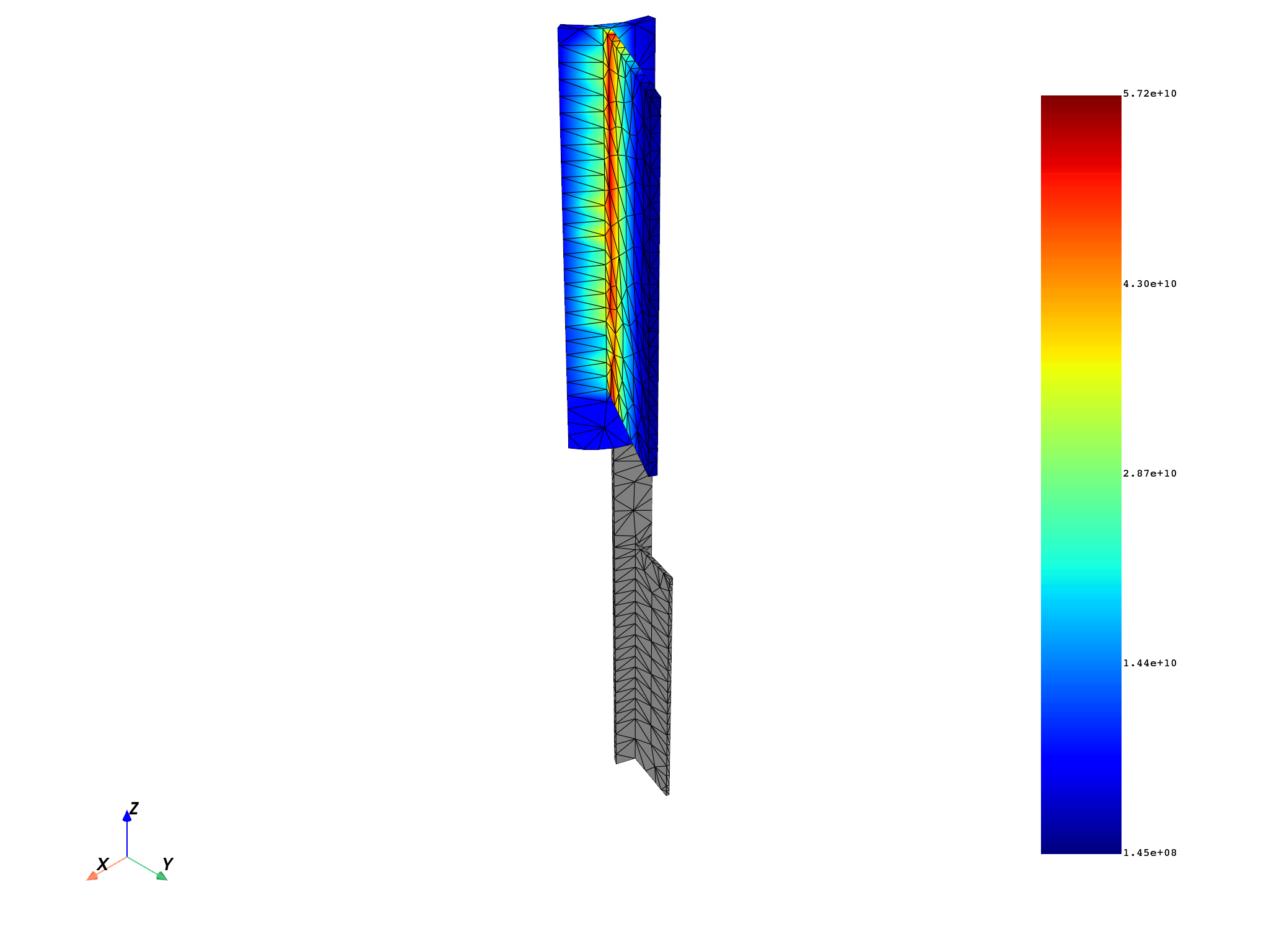
Plot result field

Plot the result field on the skin mesh:

mesh.plot(field_to_keep)

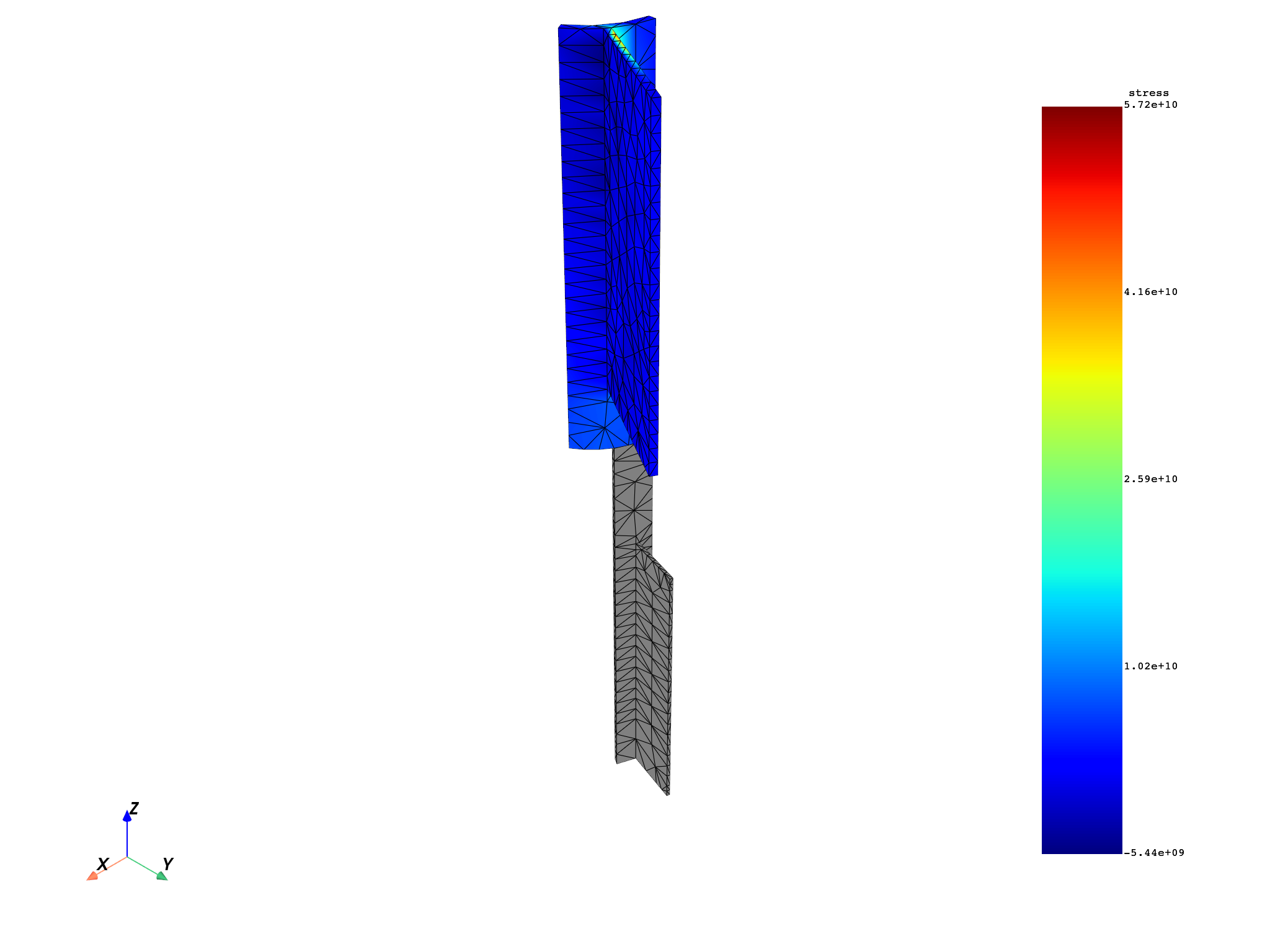
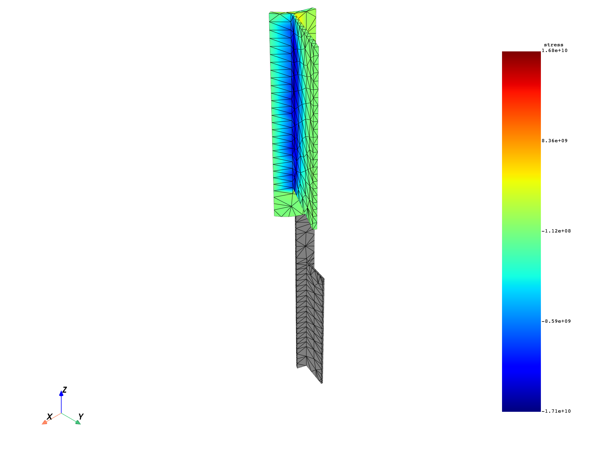
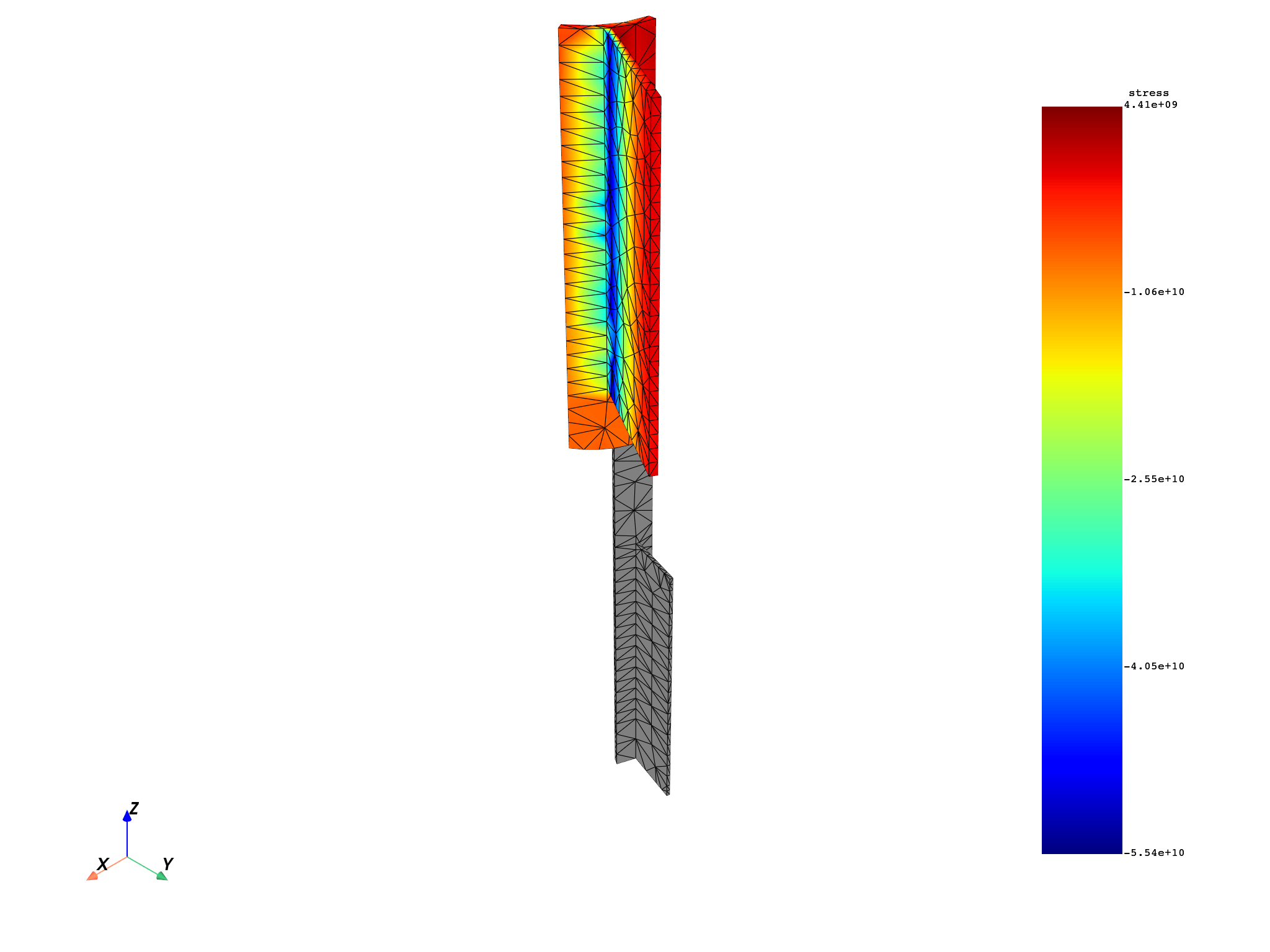
Plot initial invariants

Plot the initial invariants:

mesh.plot(principal_stress_1)
mesh.plot(principal_stress_2)
mesh.plot(principal_stress_3)

• 
• 
•