Review of available plotting commands

This example lists the different plotting commands available, shown with the arguments available.

Static Scene

Interactive Scene

Static Scene

Interactive Scene

Static Scene

Interactive Scene

Static Scene

Interactive Scene

Static Scene

Interactive Scene

Static Scene

Interactive Scene

Static Scene

Interactive Scene

Static Scene

Interactive Scene

Static Scene

Interactive Scene

Static Scene

Interactive Scene

Static Scene

Interactive Scene

DPF Model
------------------------------
Static analysis
Unit system: MKS: m, kg, N, s, V, A, degC
Physics Type: Mechanical
Available results:
     -  node_orientations: Nodal Node Euler Angles
     -  displacement: Nodal Displacement
     -  nodal_rotation: Nodal Rotation
     -  reaction_force: Nodal Reaction Force
     -  reaction_moment: Nodal Reaction Moment
     -  stress: ElementalNodal Stress
     -  elemental_volume: Elemental Volume
     -  stiffness_matrix_energy: Elemental Energy-stiffness matrix
     -  artificial_hourglass_energy: Elemental Hourglass Energy
     -  kinetic_energy: Elemental Kinetic Energy
     -  co_energy: Elemental co-energy
     -  incremental_energy: Elemental incremental energy
     -  thermal_dissipation_energy: Elemental thermal dissipation energy
     -  elastic_strain: ElementalNodal Strain
     -  elastic_strain_eqv: ElementalNodal Strain eqv
     -  element_orientations: ElementalNodal Element Euler Angles
     -  structural_temperature: ElementalNodal Structural temperature
     -  contact_status: ElementalNodal Contact Status
     -  contact_penetration: ElementalNodal Contact Penetration
     -  contact_pressure: ElementalNodal Contact Pressure
     -  contact_friction_stress: ElementalNodal Contact Friction Stress
     -  contact_total_stress: ElementalNodal Contact Total Stress
     -  contact_sliding_distance: ElementalNodal Contact Sliding Distance
     -  contact_gap_distance: ElementalNodal Contact Gap Distance
     -  contact_surface_heat_flux: ElementalNodal Total heat flux at contact surface
     -  num_surface_status_changes: ElementalNodal Contact status changes
     -  contact_fluid_penetration_pressure: ElementalNodal Fluid Penetration Pressure
------------------------------
DPF  Meshed Region:
  7079 nodes
  4220 elements
  Unit: m
  With solid (3D) elements, shell (2D) elements, shell (3D) elements
------------------------------
DPF  Time/Freq Support:
  Number of sets: 1
Cumulative     Time (s)       LoadStep       Substep
1              1.000000       1              1


([], <pyvista.plotting.plotter.Plotter object at 0x000002075656B510>)

from ansys.dpf import core as dpf
from ansys.dpf.core import examples

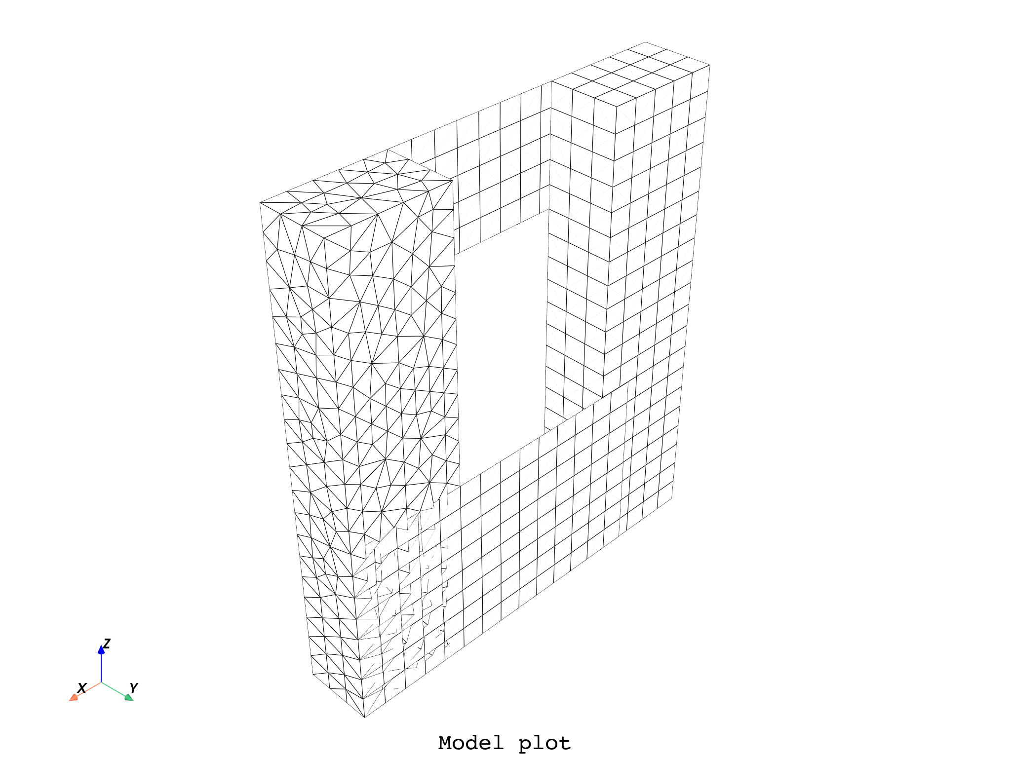
# Plot the bare mesh of a model
model = dpf.Model(examples.find_multishells_rst())
print(model)
model.plot(color="w", show_edges=True, title="Model", text="Model plot")
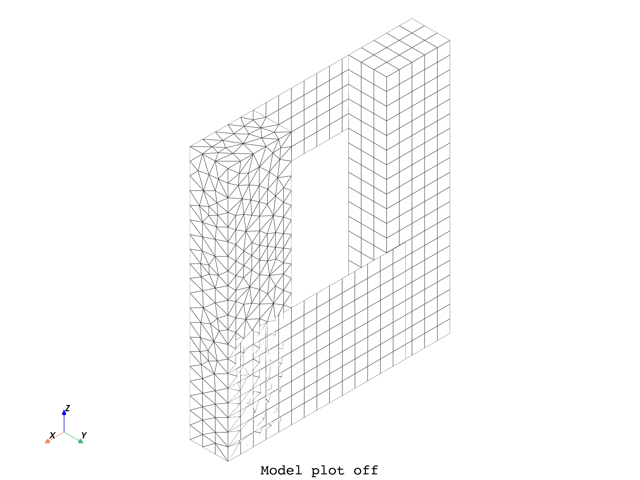
# # Additional PyVista kwargs are supported, such as:
model.plot(
    off_screen=True,
    notebook=False,
    screenshot="model_plot.png",
    title="Model",
    text="Model plot off",
    parallel_projection=True,
    zoom=2.0,
)

# Notes:
# - To make screenshots, use "screenshot" as well as "notebook=False" if on a Jupyter notebook.
# - The "off_screen" keyword only works when "notebook=False" to prevent the GUI from appearing.


# Plot a field on its supporting mesh
stress = model.results.stress()
# We request the stress as nodal to bypass a bug for DPF 2025 R1 and below
# which prevents from plotting ElementalNodal data on shells
stress.inputs.requested_location.connect(dpf.locations.nodal)
fc = stress.outputs.fields_container()
field = fc[0]
field.plot(notebook=False, shell_layers=None, show_axes=True, title="Field", text="Field plot")
# # Additional PyVista kwargs are supported, such as:
field.plot(
    off_screen=True,
    notebook=False,
    screenshot="field_plot.png",
    title="Field",
    text="Field plot off",
)
#
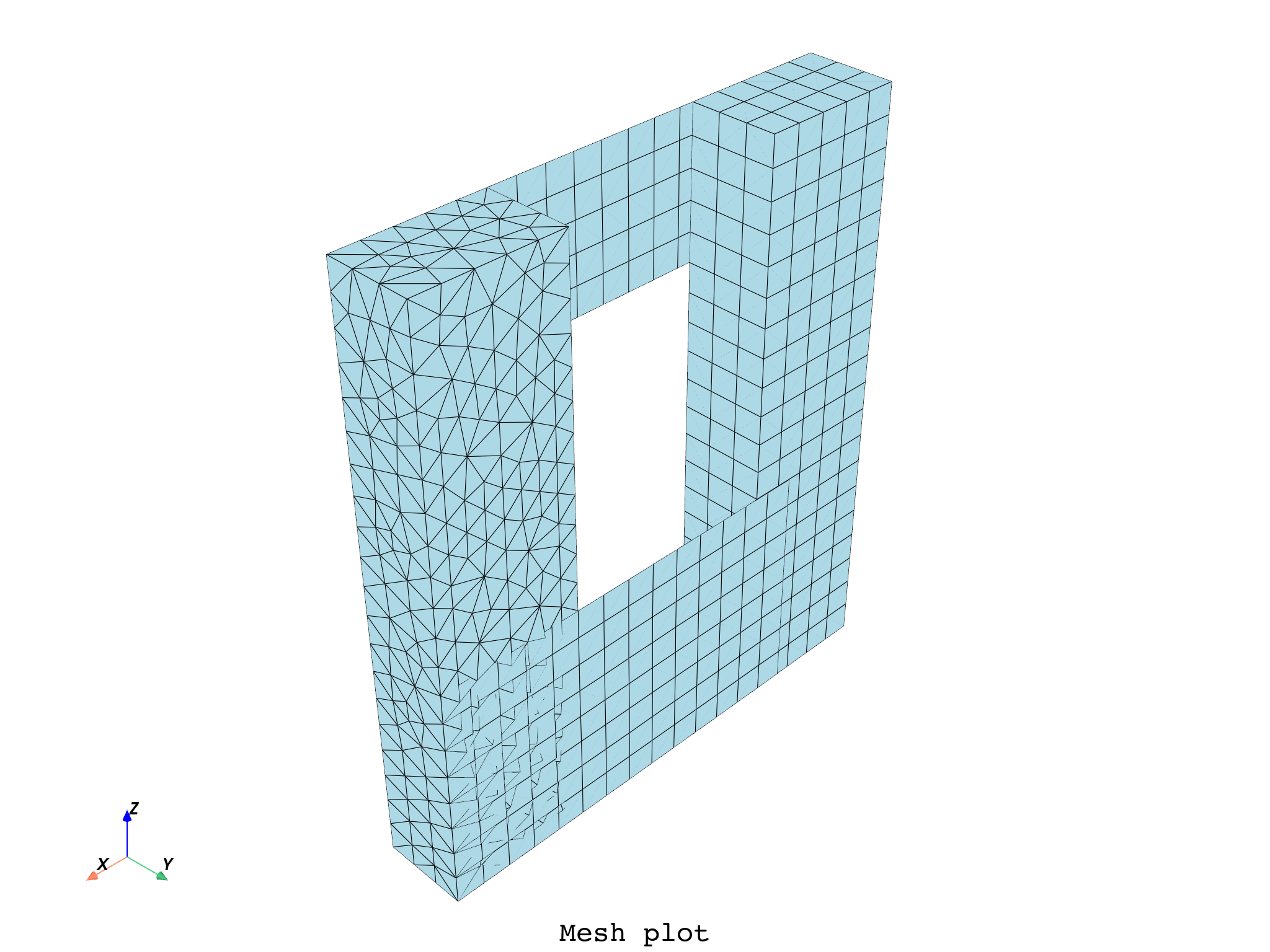
# # Alternatively one can plot the MeshedRegion associated to the model
mesh = model.metadata.meshed_region
mesh.plot(
    field_or_fields_container=None,
    shell_layers=None,
    show_axes=True,
    title="Mesh fc None",
    text="Mesh plot",
)
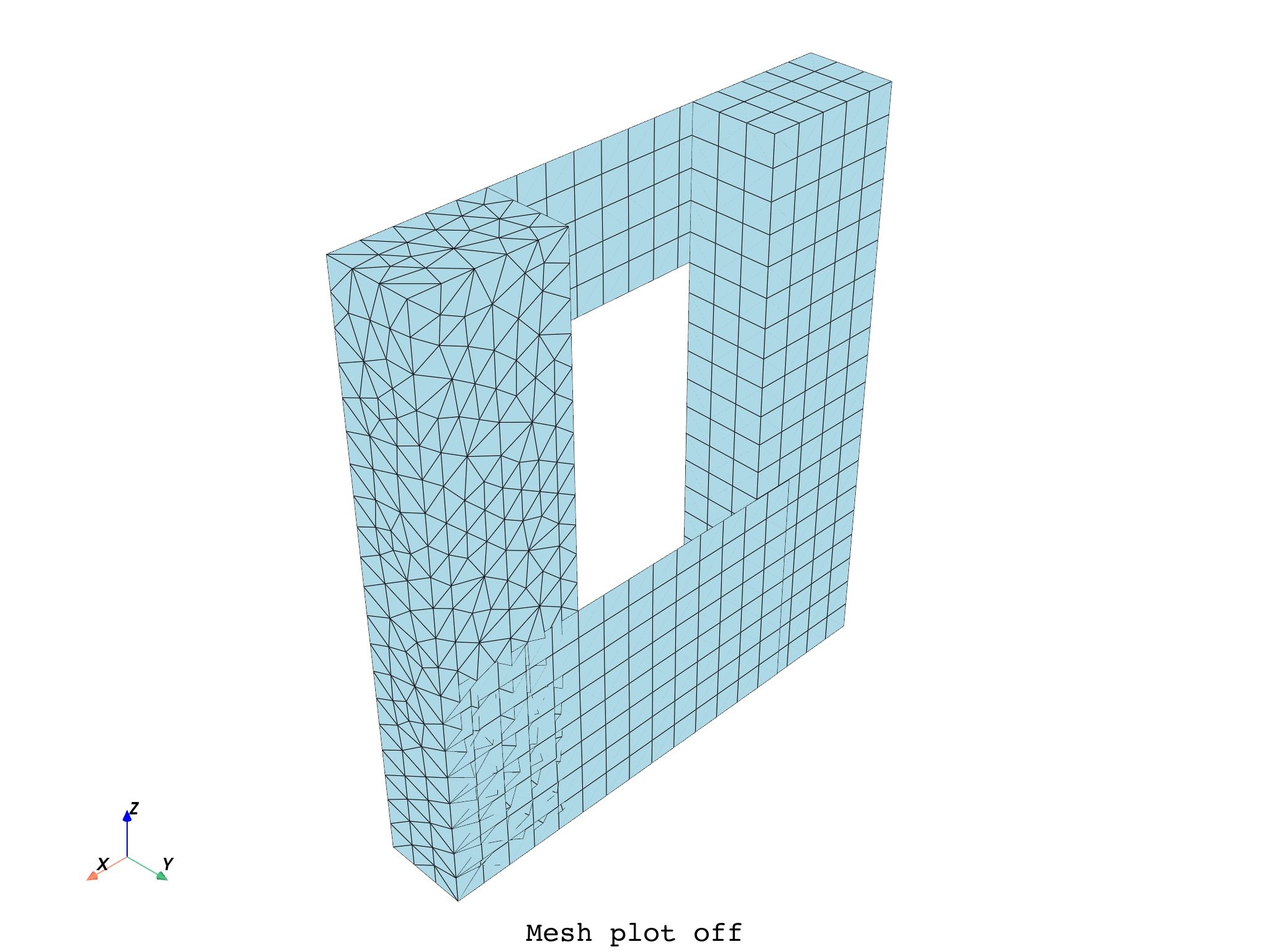
# Additional PyVista kwargs are supported, such as:
mesh.plot(
    off_screen=True,
    notebook=False,
    screenshot="mesh_plot.png",
    title="Mesh",
    text="Mesh plot off",
)
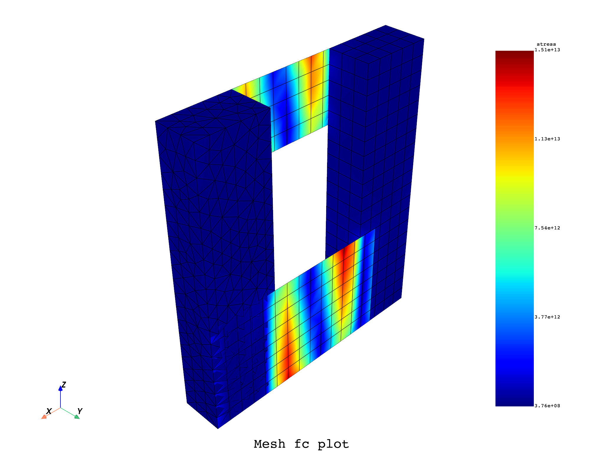
# A fields_container or a specific field can be given to plot on the mesh.
mesh.plot(
    field_or_fields_container=fc,
    title="Mesh with fields container",
    text="Mesh fc plot",
)
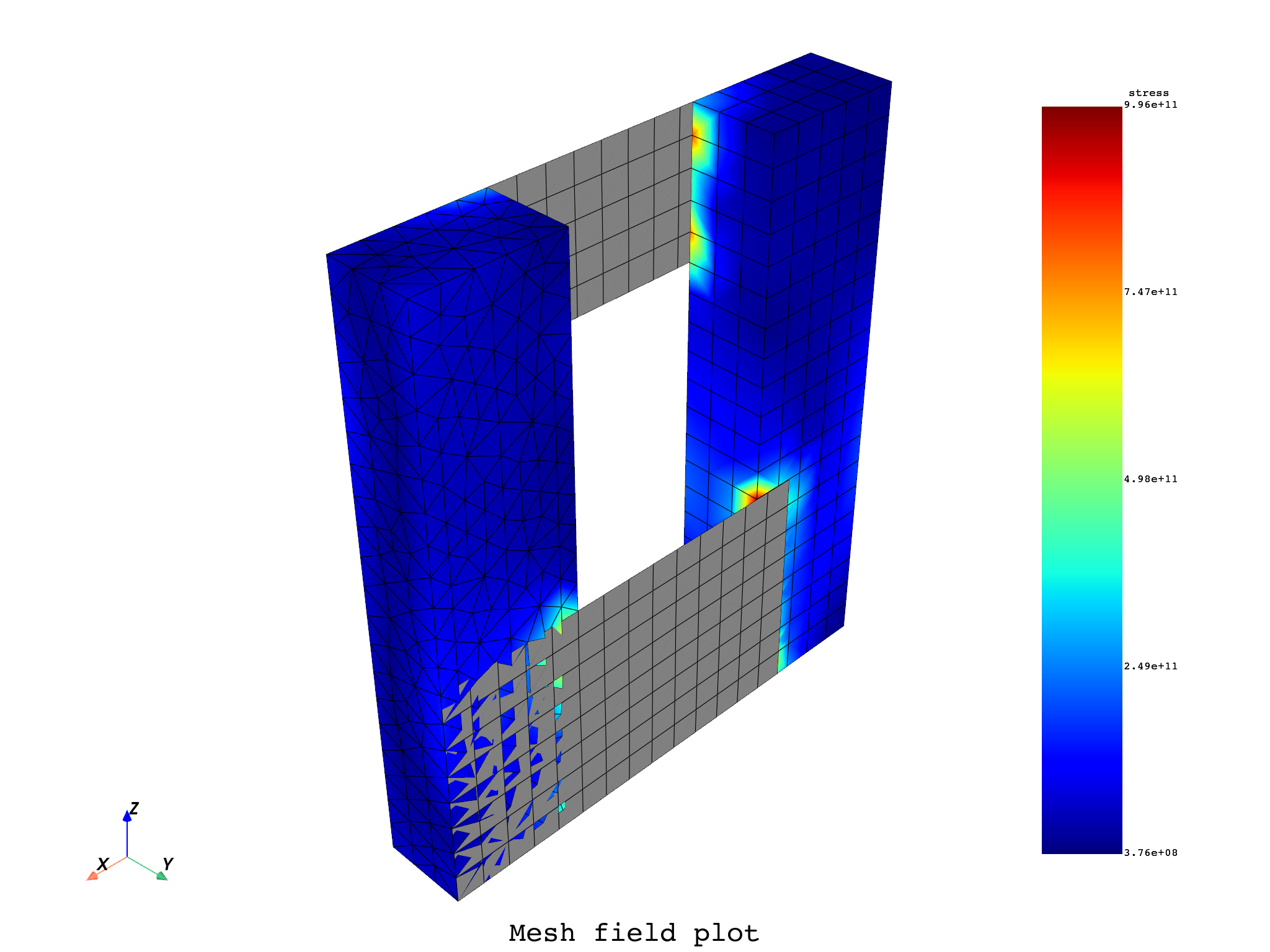
mesh.plot(field_or_fields_container=field, title="Mesh with field", text="Mesh field plot")


# ##############################################################################################
# # This next section requires a Premium context to be active du to the ``split_mesh`` operator.
# # Comment this last part to run the example as Entry.

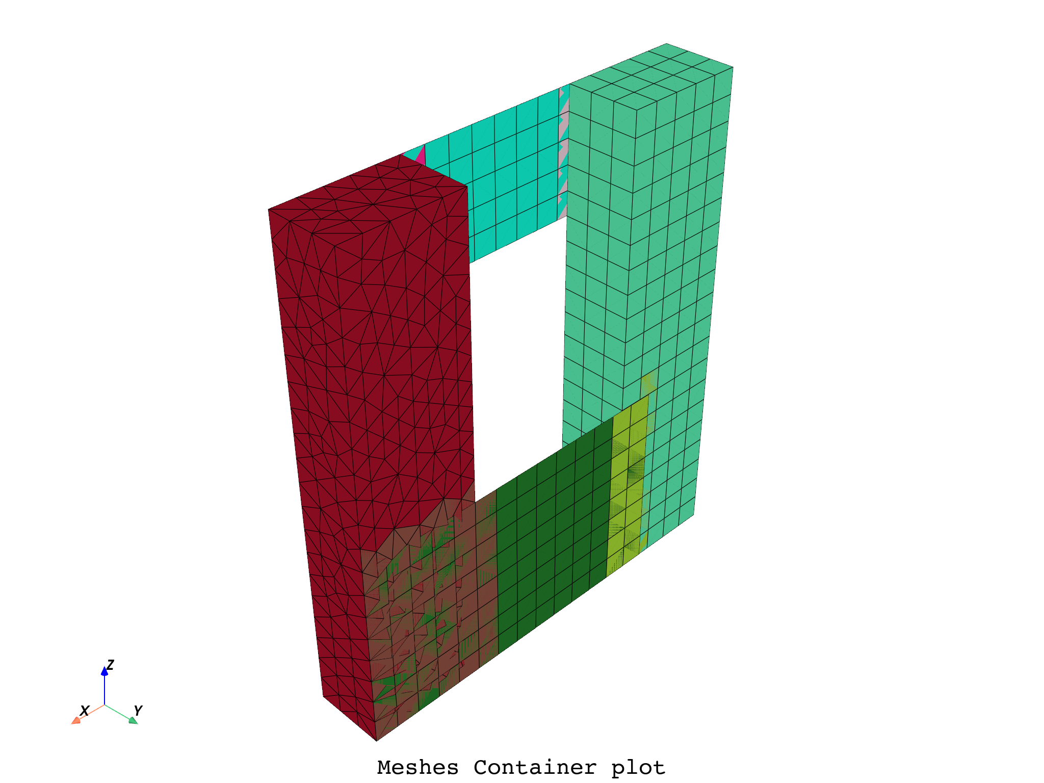
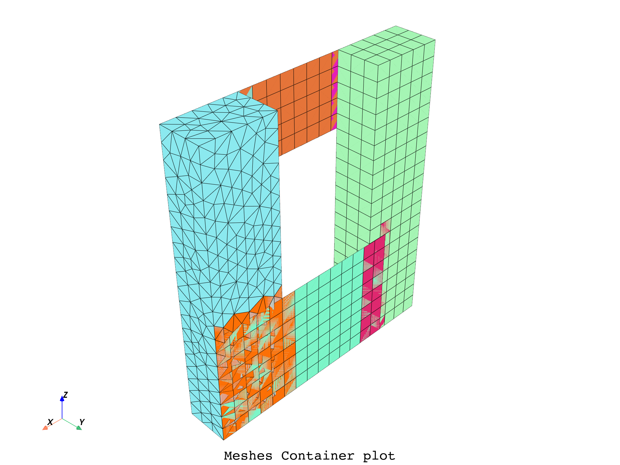
# One can also plot a MeshesContainer. Here our mesh is split by material.
split_mesh_op = dpf.Operator("split_mesh")
split_mesh_op.connect(7, mesh)
split_mesh_op.connect(13, "mat")
meshes_cont = split_mesh_op.get_output(0, dpf.types.meshes_container)
meshes_cont.plot(title="Meshes Container", text="Meshes Container plot")
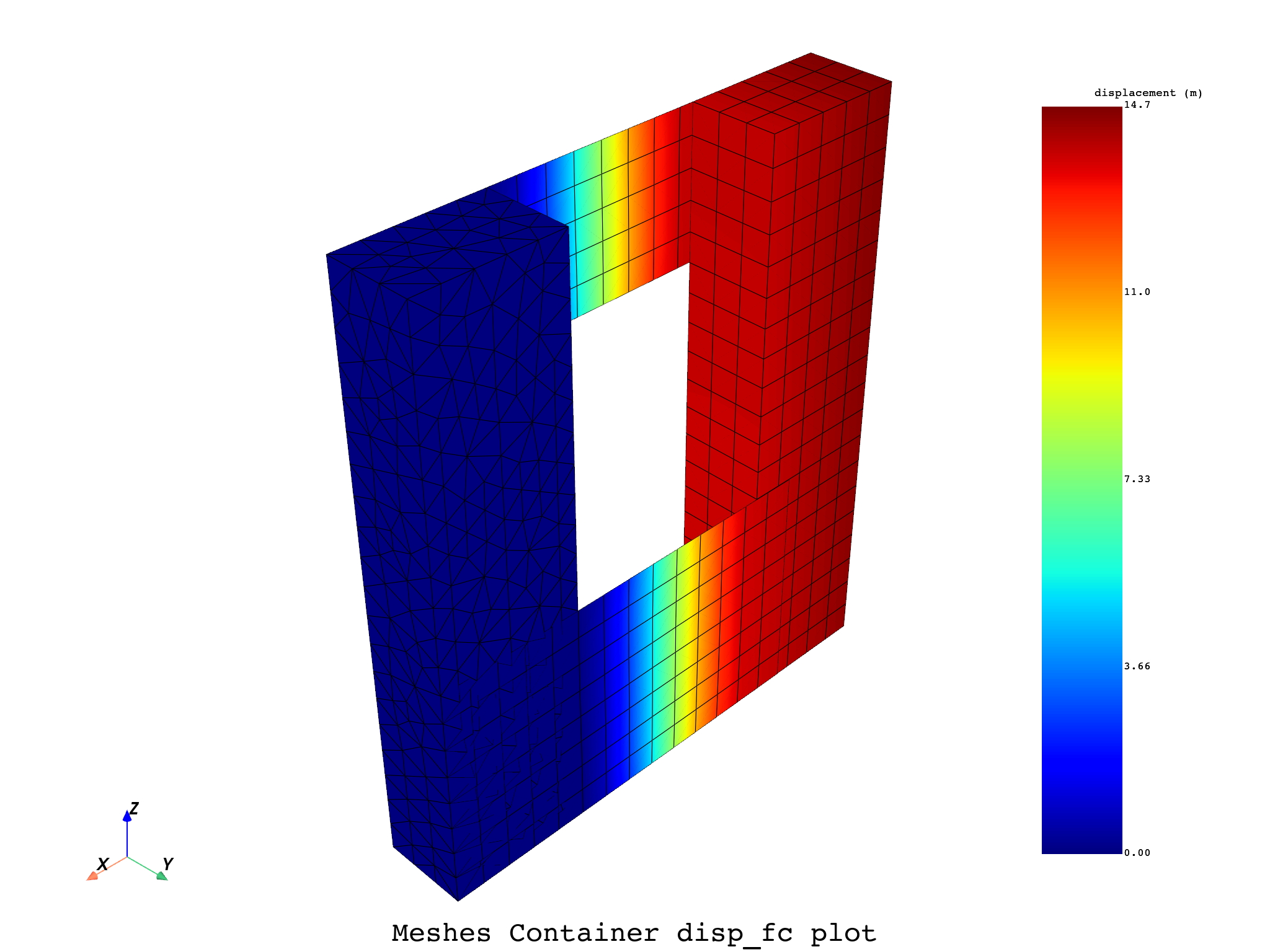
# A fields_container can be given as input, with results on each part of our split mesh.
disp_op = dpf.Operator("U")
disp_op.connect(7, meshes_cont)
ds = dpf.DataSources(examples.find_multishells_rst())
disp_op.connect(4, ds)
disp_fc = disp_op.outputs.fields_container()
meshes_cont.plot(disp_fc, title="Meshes Container disp_fc", text="Meshes Container disp_fc plot")
# Additional PyVista kwargs are supported, such as:
meshes_cont.plot(
    off_screen=True,
    notebook=False,
    screenshot="meshes_cont_plot.png",
    title="Meshes Container",
    text="Meshes Container plot",
)