Note
Go to the end to download the full example code.
Load case combination for principal stress#
This example shows how to get a principal stress load case combination using DPF And highlight min/max values in the plot.
Import the ansys.dpf.core module, included examples file, and the DpfPlotter
module.
from ansys.dpf import core as dpf
from ansys.dpf.core import examples
from ansys.dpf.core.plotter import DpfPlotter
Open an example and print the Model object. The
Model class helps to organize access
methods for the result by keeping track of the operators and data sources
used by the result file.
Printing the model displays this metadata:
Analysis type
Available results
Size of the mesh
Number of results
model = dpf.Model(examples.find_msup_transient())
print(model)
DPF Model
------------------------------
Transient analysis
Unit system: MKS: m, kg, N, s, V, A, degC
Physics Type: Mechanical
Available results:
     -  node_orientations: Nodal Node Euler Angles
     -  displacement: Nodal Displacement
     -  velocity: Nodal Velocity
     -  acceleration: Nodal Acceleration
     -  reaction_force: Nodal Reaction Force
     -  stress: ElementalNodal Stress
     -  elemental_volume: Elemental Volume
     -  stiffness_matrix_energy: Elemental Energy-stiffness matrix
     -  artificial_hourglass_energy: Elemental Hourglass Energy
     -  kinetic_energy: Elemental Kinetic Energy
     -  co_energy: Elemental co-energy
     -  incremental_energy: Elemental incremental energy
     -  thermal_dissipation_energy: Elemental thermal dissipation energy
     -  elastic_strain: ElementalNodal Strain
     -  elastic_strain_eqv: ElementalNodal Strain eqv
------------------------------
DPF  Meshed Region:
  393 nodes
  40 elements
  Unit: m
  With solid (3D) elements
------------------------------
DPF  Time/Freq Support:
  Number of sets: 20
Cumulative     Time (s)       LoadStep       Substep
1              0.010000       1              1
2              0.020000       1              2
3              0.030000       1              3
4              0.040000       1              4
5              0.050000       1              5
6              0.060000       1              6
7              0.070000       1              7
8              0.080000       1              8
9              0.090000       1              9
10             0.100000       1              10
11             0.110000       1              11
12             0.120000       1              12
13             0.130000       1              13
14             0.140000       1              14
15             0.150000       1              15
16             0.160000       1              16
17             0.170000       1              17
18             0.180000       1              18
19             0.190000       1              19
20             0.200000       1              20
Get the stress tensor and connect time scoping.
Make sure that you define dpf.locations.nodal as the scoping location because
labels are supported only for nodal results.
stress_tensor = model.results.stress()
time_scope = dpf.Scoping()
time_scope.ids = [1, 2]
stress_tensor.inputs.time_scoping.connect(time_scope)
stress_tensor.inputs.requested_location.connect(dpf.locations.nodal)
This code performs solution combination on two load cases, LC1 and LC2. You can access individual load cases as the fields of a fields container for the stress tensor.
field_lc1 = stress_tensor.outputs.fields_container()[0]
field_lc2 = stress_tensor.outputs.fields_container()[1]

# Scale LC2 to -1.
stress_tensor_lc2_sc = dpf.operators.math.scale(field=field_lc2, weights=-1.0)
Add load cases.
stress_tensor_combi = dpf.operators.math.add(fieldA=field_lc1, fieldB=stress_tensor_lc2_sc)
Principal stresses are the Eigenvalues of the stress tensor. Use principal invariants to get S1, S2, and S3.
p_inv = dpf.operators.invariant.principal_invariants()
p_inv.inputs.field.connect(stress_tensor_combi)
Print S1 (maximum principal stress).
print(p_inv.outputs.field_eig_1().data)
[ 9.89969387e+05  9.86979842e+05  6.46045019e+05  6.48932208e+05
  1.56976611e+04  2.38335566e+03  2.41021560e+03  1.55569949e+04
  6.46045018e+05  9.86979841e+05  2.41021536e+03  2.38335517e+03
  1.40298687e+06  1.40006022e+06  1.51284404e+04  2.32609985e+03
  1.40006022e+06  2.32609969e+03  1.88584658e+06  1.88308883e+06
  1.40245029e+04  2.28989834e+03  1.88308883e+06  2.28989838e+03
  2.43323154e+06  2.43097276e+06  1.13710605e+04  1.92191439e+03
  2.43097276e+06  1.92191428e+03  3.03740836e+06  3.03544790e+06
  8.36913086e+03  5.11051169e+03  3.03544790e+06  5.11051165e+03
  3.68414662e+06  3.68923438e+06 -4.49507141e+03 -3.86970389e+03
  3.68923438e+06 -3.86970407e+03  4.37493535e+06  4.36801081e+06
  4.62750323e+04  6.45366758e+04  4.36801080e+06  6.45366739e+04
  5.00024912e+06  5.15363818e+06 -1.72558410e+05 -1.68506344e+05
  5.15363818e+06 -1.68506347e+05  5.34040385e+06  6.25295625e+06
  9.15169741e+05  5.86694135e+05  6.25295625e+06  5.86694135e+05
  8.19942478e+06  5.11230070e+06 -3.42443463e+06 -1.72869110e+06
  5.11230070e+06 -1.72869110e+06  3.07108105e+03  4.85742708e+02
  2.08121801e+03  4.51329102e+03  1.15257484e+04  1.08729694e+04
  1.48084273e+02  6.58067584e+01  2.08121700e+03  4.85743242e+02
  1.48084276e+02  1.08729663e+04  3.99734802e+02  2.84198603e+02
  3.98308935e+04  3.99596263e+04  2.84199027e+02  3.99596267e+04
  8.05592976e+00  7.63702585e+01  7.02630967e+04  7.11528217e+04
  7.63704604e+01  7.11528219e+04  4.08416639e+00  8.37761486e+01
  8.97598110e+04  9.14268559e+04  8.37761220e+01  9.14268560e+04
  5.48381675e+00  1.42362400e+02  8.58241342e+04  8.84204337e+04
  1.42362254e+02  8.84204335e+04  1.36280987e+01  1.13419159e+03
  4.68127641e+04  5.12948274e+04  1.13419050e+03  5.12948265e+04
  3.78823067e+04  3.90599658e+04  1.20048086e+04  5.25881723e+03
  3.90599642e+04  5.25881571e+03  1.77336944e+05  1.75477888e+05
  1.36475040e+04  2.76759779e+03  1.75477887e+05  2.76759705e+03
  3.79160579e+05  3.76590414e+05  1.48577178e+04  2.47204930e+03
  3.76590413e+05  2.47204876e+03  9.87954234e+05  8.16487441e+05
  6.46963602e+05  8.19450620e+05  8.32083289e+03  2.37183132e+03
  8.24629107e+03  1.56273280e+04  4.22633967e+03  2.09163879e+04
  1.69460011e+04  3.38679027e+03  6.46963601e+05  8.16487441e+05
  9.87954234e+05  8.24629092e+03  2.37183096e+03  8.32083271e+03
  1.69460004e+04  2.09163879e+04  1.40100768e+06  1.19350278e+06
  1.19647800e+06  8.06338005e+03  2.33617878e+03  1.54130508e+04
  5.06746339e+03  2.48394848e+04  1.19350278e+06  1.40100768e+06
  2.33617846e+03  8.06337997e+03  2.48394841e+04  1.88395758e+06
  1.64156177e+06  1.64441663e+06  7.53335722e+03  2.29511028e+03
  1.45764717e+04  5.88761468e+03  2.85398928e+04  1.64156177e+06
  1.88395758e+06  2.29511022e+03  7.53335719e+03  2.85398937e+04
  2.43161333e+06  2.15701918e+06  2.15953899e+06  6.20773016e+03
  2.02784724e+03  1.26977817e+04  6.67395032e+03  3.18340564e+04
  2.15701918e+06  2.43161333e+06  2.02784721e+03  6.20773009e+03
  3.18340564e+04  3.03594055e+06  2.73320351e+06  2.73531989e+06
  5.60676164e+03  2.72710830e+03  9.87009570e+03  7.46575696e+03
  3.45048447e+04  2.73320351e+06  3.03594055e+06  2.72710810e+03
  5.60676149e+03  3.45048427e+04  3.68631143e+06  3.36231959e+06
  3.36077747e+06 -4.64521947e+03 -4.02685627e+00  1.93702972e+03
  8.47413202e+03  3.63891780e+04  3.36231959e+06  3.68631143e+06
 -4.02705347e+00 -4.64521954e+03  3.63891782e+04  4.37097945e+06
  4.02861843e+06  4.02954094e+06  5.48856888e+04  2.66267135e+04
  1.70544403e+04  9.30881824e+03  3.76058067e+04  4.02861843e+06
  4.37097945e+06  2.66267128e+04  5.48856879e+04  3.76058038e+04
  5.07685002e+06  4.75984186e+06  4.68757240e+06 -1.70825434e+05
 -5.92324427e+04 -6.58878990e+04  3.01483062e+04  2.40997043e+04
  4.75984186e+06  5.07685002e+06 -5.92324444e+04 -1.70825436e+05
  2.40996713e+04  5.79541432e+06  5.70261123e+06  5.17030113e+06
  7.41483955e+05  1.80559706e+05  3.68553935e+05  1.21181294e+04
  5.77464735e+04  5.70261123e+06  5.79541432e+06  1.80559705e+05
  7.41483955e+05  5.77464732e+04  6.76007838e+06  6.55138588e+06
  5.60950676e+06 -1.27232574e+06 -2.58721655e+06 -6.39421513e+05
  4.13265031e+05  4.45501864e+05  5.60950676e+06  6.55138588e+06
 -6.39421513e+05 -2.58721655e+06  4.45501864e+05  1.61943216e+03
  3.10965572e+02  2.25636060e+03  3.79218604e+03  1.10854389e+04
  4.53912469e+03  9.07955770e+01  4.93947446e+03  3.68349703e+02
  1.18342832e+03  3.42938262e+01  4.05442820e+01  2.25636052e+03
  3.10965881e+02  1.61943240e+03  9.07956839e+01  4.53912372e+03
  1.10854373e+04  3.42939134e+01  1.18342850e+03  2.65656153e+02
  3.16995504e+02  1.73540793e+03  3.98371654e+04  2.53482084e+04
  2.56765725e+04  4.87884515e+02  1.64634854e+03  3.16995859e+02
  2.65656367e+02  2.53482069e+04  3.98371655e+04  1.64634882e+03
  1.20868138e+01  1.53332553e+02  8.34477875e+00  7.06858860e+04
  5.55323220e+04  5.50465228e+04  4.32272090e+02  1.40242459e+03
  1.53332839e+02  1.20867966e+01  5.55323222e+04  7.06858860e+04
  1.40242520e+03  6.52978300e+00  6.11437148e+01  5.82177773e+00
  9.05926824e+04  8.12697662e+04  8.00112056e+04  2.33592980e+02
  4.52921390e+02  6.11437305e+01  6.52982809e+00  8.12697663e+04
  9.05926824e+04  4.52922199e+02  1.01781946e+01  1.06177194e+02
  4.46460174e+00  8.70987991e+04  8.98867421e+04  8.77916532e+04
  1.04133938e+02  1.18550598e+03  1.06177120e+02  1.01781534e+01
  8.98867421e+04  8.70987990e+04  1.18550523e+03  8.92616048e+01
  3.61429147e+02  7.74169288e+00  4.88073415e+04  6.96187475e+04
  6.63166348e+04  5.69214730e+02  3.42490749e+03  3.61428542e+02
  8.92614996e+01  6.96187470e+04  4.88073411e+04  3.42490700e+03
  3.71947352e+04  7.66384058e+03  1.66212838e+02  7.00641342e+03
  1.58464803e+04  1.09997182e+04  1.14790002e+03  6.21377392e+03
  7.66383803e+03  3.71947343e+04  1.58464779e+04  7.00641255e+03
  6.21377387e+03  1.75780678e+05  1.06374478e+05  1.07603370e+05
  7.35047360e+03  3.11936342e+03  1.28261563e+04  1.82375472e+03
  9.46675704e+03  1.06374477e+05  1.75780677e+05  3.11936250e+03
  7.35047326e+03  9.46675639e+03  3.77331700e+05  2.75920917e+05
  2.78248027e+05  7.90102104e+03  2.50682872e+03  1.42526109e+04
  2.57757172e+03  1.30834902e+04  2.75920916e+05  3.77331700e+05
  2.50682813e+03  7.90102076e+03  1.30834897e+04  5.11273760e+05
  5.14046095e+05  2.39727952e+03  1.52073563e+04  5.11273759e+05
  2.39727916e+03]
Get the meshed region.
mesh_set = model.metadata.meshed_region
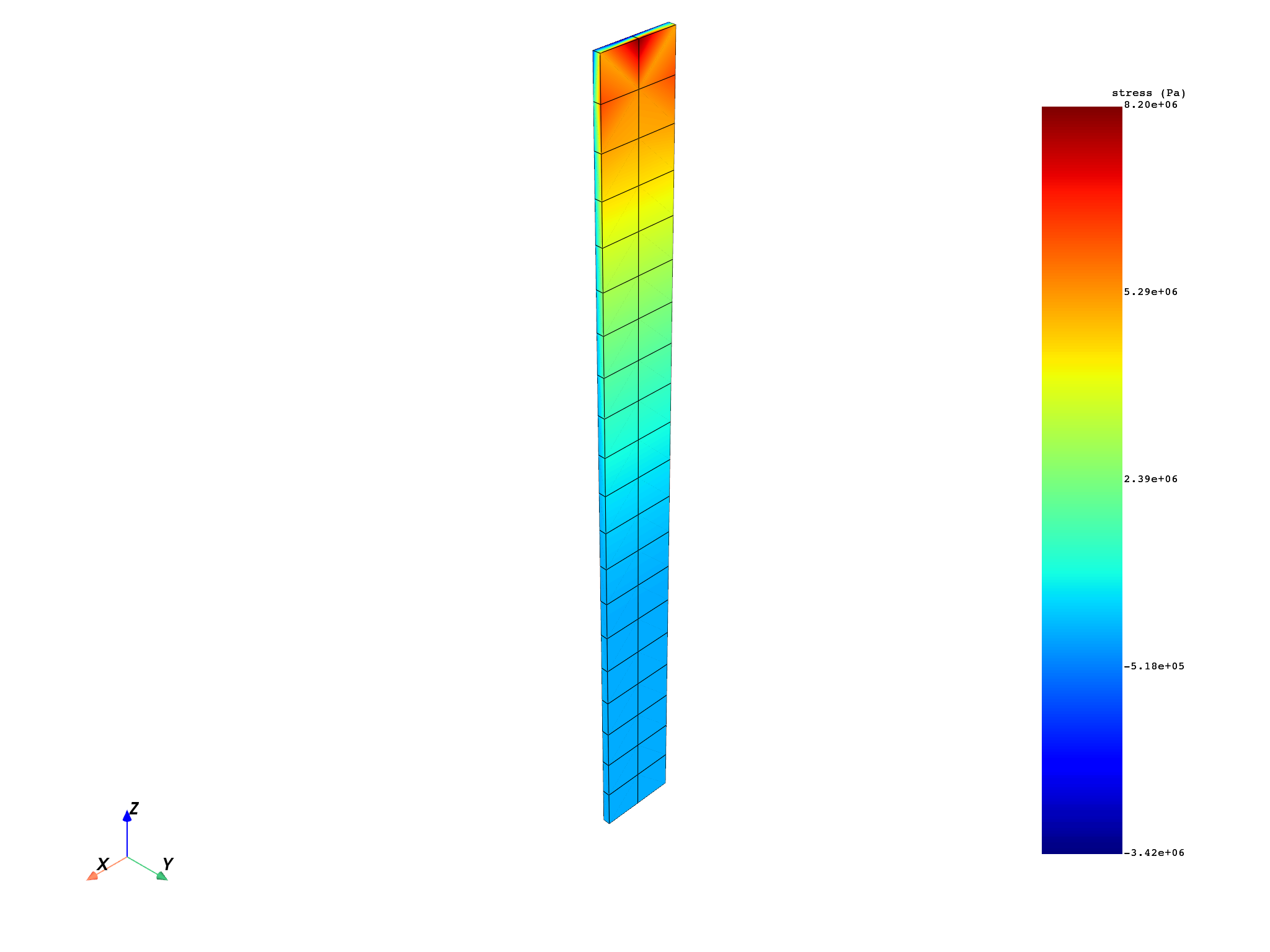
Plot the results on the mesh.
The label_text_size and label_point_size arguments control the font
size of the label.
plot = DpfPlotter()
plot.add_field(p_inv.outputs.field_eig_1(), meshed_region=mesh_set)

# You can set the camera positions using the ``cpos`` argument.
# The three tuples in the list for the ``cpos`` argument represent the camera
# position, focal point, and view respectively.
plot.show_figure(show_axes=True)
([], <pyvista.plotting.plotter.Plotter object at 0x00000264A3093E10>)
Total running time of the script: (0 minutes 1.852 seconds)