Calculate the number of cycles to fatigue failure

This example shows how to generate and use a result file to calculate the cycles to failure result for a simple model.

Material data is manually imported, Structural Steel from Ansys Mechanical:

• Youngs Modulus (youngsSteel)

• Poisson’s Ratio (prxySteel)

• SN curve (sn_data)

The first step is to generate a simple model with high stress and save the results .rst file locally to myDir (default is “C:\temp”). For this, we provide a short pyMAPDL script.

The second step uses PyDPF-Core to generate the cycles to failure result:

The locally saved .rst file is imported and plotted.

Then the von Mises stress is generated and plotted with DPF operators.

The NumPy python package is then used to interpolate the cycles to failure values.

The nodal von Mises equivalent stress value is used in the interpolation.

(Note that the cycles to failure data must be manipulated to use NumPy interpolation)

An empty field is then created and filled with the resulting cycles to failure values.

The cycles to failure result is finally plotted.

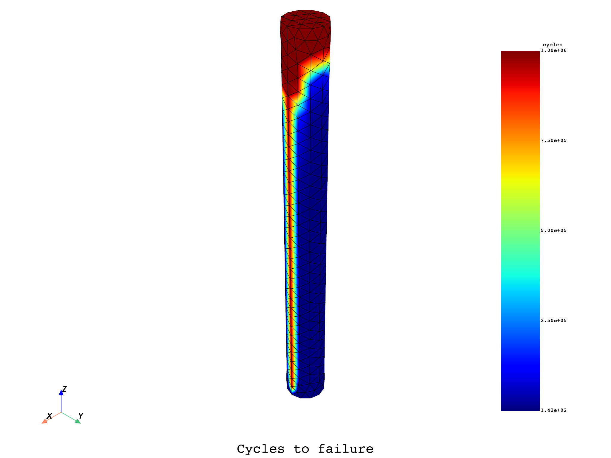
The cycles to failure result is the (interpolated) negative of the stress result. The higher the stress result, the lower the number of cycles to failure.

from ansys.dpf import core as dpf
from ansys.dpf.core import examples
import numpy as np

The first step is to generate a simple model with high stress

# # Material parameters from Ansys Mechanical Structural Steel
youngsSteel = 200e9
prxySteel = 0.3
sn_data = np.empty((11, 2))  # initialize empty np matrix
sn_data[:, 0] = [10, 20, 50, 100, 200, 2000, 10000, 20000, 1e5, 2e5, 1e6]
sn_data[:, 1] = [
    3.999e9,
    2.8327e9,
    1.896e9,
    1.413e9,
    1.069e9,
    4.41e8,
    2.62e8,
    2.14e8,
    1.38e8,
    1.14e8,
    8.62e7,
]

The .rst file used is already available, but can be obtained using the short pyMAPDL code below:

# # ### Launch pymapdl to generate rst file in myDir
# from ansys.mapdl.core import launch_mapdl
# import os
#
#
# mapdl = launch_mapdl()
# mapdl.prep7()
# # Model
# mapdl.cylind(0.5, 0, 10, 0)
# mapdl.mp("EX", 1, youngsSteel)
# mapdl.mp("PRXY", 1, prxySteel)
# mapdl.mshape(key=1, dimension='3d')
# mapdl.et(1, "SOLID186")
# mapdl.esize(0.3)
# mapdl.vmesh('ALL')
#
# # #### Boundary Conditions: fixed constraint
# mapdl.nsel(type_='S', item='LOC', comp='Z', vmin=0)
# mapdl.d("all", "all")
# mapdl.nsel(type_='S', item='LOC', comp='Z', vmin=10)
# nnodes = mapdl.get("NumNodes", "NODE", 0, "COUNT")
# mapdl.f(node="ALL", lab="fy", value=-13e6 / nnodes)
# mapdl.allsel()
#
# # #### Solve
# mapdl.run("/SOLU")
# sol_output = mapdl.solve()
# rst = os.path.join(mapdl.directory, 'file.rst')
# mapdl.exit()
# print('apdl model solved.')

PyDPF-Core is then used to post-process the .rst file to estimate the cycles to failure.

# Comment the following line if solving the MAPDL problem first.
rst = examples.download_cycles_to_failure()

# Import the result as a DPF Model object.
model = dpf.Model(rst)
print(model)

DPF Model
------------------------------
Static analysis
Unit system: Undefined
Physics Type: Mechanical
Available results:
     -  displacement: Nodal Displacement
     -  reaction_force: Nodal Force
     -  elemental_summable_miscellaneous_data: Elemental Elemental Summable Miscellaneous Data
     -  element_nodal_forces: ElementalNodal Element nodal Forces
     -  stress: ElementalNodal Stress
     -  elemental_volume: Elemental Volume
     -  stiffness_matrix_energy: Elemental Energy-stiffness matrix
     -  artificial_hourglass_energy: Elemental Hourglass Energy
     -  thermal_dissipation_energy: Elemental thermal dissipation energy
     -  kinetic_energy: Elemental Kinetic Energy
     -  co_energy: Elemental co-energy
     -  incremental_energy: Elemental incremental energy
     -  elastic_strain: ElementalNodal Strain
     -  thermal_strain: ElementalNodal Thermal Strains
     -  thermal_strains_eqv: ElementalNodal Thermal Strains eqv
     -  swelling_strains: ElementalNodal Swelling Strains
     -  element_euler_angles: ElementalNodal Element Euler Angles
     -  structural_temperature: ElementalNodal Structural temperature
------------------------------
DPF  Meshed Region:
  4102 nodes
  2356 elements
  Unit:
  With solid (3D) elements
------------------------------
DPF  Time/Freq Support:
  Number of sets: 1
Cumulative     Time (s)       LoadStep       Substep
1              1.000000       1              1

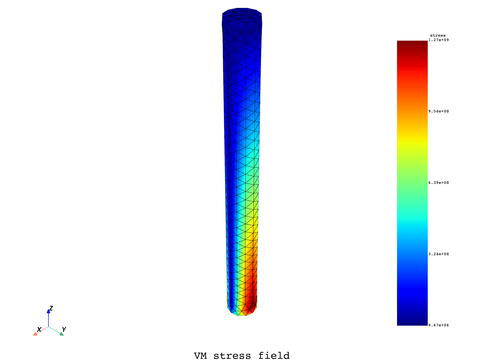
Get the von mises equivalent stress, requires an operator.

s_eqv_op = dpf.operators.result.stress_von_mises(data_sources=model)
vm_stress_fc = s_eqv_op.eval()
vm_stress_field = vm_stress_fc[0]
vm_stress_field.plot(text="VM stress field")

Use NumPy to interpolate the results.

# Inverse the sn_data
x_values = sn_data[:, 1][::-1]  # the x values are the stress ranges in ascending order
y_values = sn_data[:, 0][::-1]  # y values are inverted cycles to failure

# Interpolate cycles to failure for the VM values
cycles_to_failure = np.interp(vm_stress_field.data, x_values, y_values)

Generate a cycles_to_failure DPF Field

# Create an empty field
cycles_to_failure_field = dpf.Field(
    nentities=len(vm_stress_field.scoping),
    nature=dpf.natures.scalar,
    location=dpf.locations.nodal,
)
# Populate the field
cycles_to_failure_field.scoping = vm_stress_field.scoping
cycles_to_failure_field.meshed_region = vm_stress_field.meshed_region
cycles_to_failure_field.data = cycles_to_failure

# Plot the field
sargs = dict(title="cycles", fmt="%.2e")
cycles_to_failure_field.plot(text="Cycles to failure", scalar_bar_args=sargs)