Stress gradient normal to a defined node

This example shows how to plot a stress gradient normal to a selected node. Because the example is based on creating a path along the normal, the selected node must be on the surface of the geometry. A path is created of a defined length.

Import the DPF-Core module as dpf and import the included examples file and DpfPlotter.

import matplotlib.pyplot as plt

from ansys.dpf import core as dpf
from ansys.dpf.core import examples
from ansys.dpf.core import operators as ops
from ansys.dpf.core.plotter import DpfPlotter

Open an example and print out the Model object. The Model class helps to organize access methods for the result by keeping track of the operators and data sources used by the result file.

Printing the model displays:

• Analysis type

• Available results

• Size of the mesh

• Number of results

• Unit

path = examples.download_hemisphere()
model = dpf.Model(path)
print(model)

DPF Model
------------------------------
Static analysis
Unit system: NMM: mm, ton, N, s, mV, mA, degC
Physics Type: Mechanical
Available results:
     -  displacement: Nodal Displacement
     -  reaction_force: Nodal Force
     -  stress: ElementalNodal Stress
     -  elemental_volume: Elemental Volume
     -  stiffness_matrix_energy: Elemental Energy-stiffness matrix
     -  artificial_hourglass_energy: Elemental Hourglass Energy
     -  thermal_dissipation_energy: Elemental thermal dissipation energy
     -  kinetic_energy: Elemental Kinetic Energy
     -  co_energy: Elemental co-energy
     -  incremental_energy: Elemental incremental energy
     -  elastic_strain: ElementalNodal Strain
     -  element_euler_angles: ElementalNodal Element Euler Angles
     -  structural_temperature: ElementalNodal Structural temperature
------------------------------
DPF  Meshed Region:
  10741 nodes
  3011 elements
  Unit: mm
  With solid (3D) elements
------------------------------
DPF  Time/Freq Support:
  Number of sets: 1
Cumulative     Time (s)       LoadStep       Substep
1              1.000000       1              1

Define the node ID normal to plot the a stress gradient

node_id = 1928

Print the mesh unit

unit = model.metadata.meshed_region.unit
print("Unit: %s" % unit)

Unit: mm

depth defines the length/depth that the path penetrates to. While defining depth make sure you use the correct mesh unit. delta defines distance between consecutive points on the path.

depth = 10  # in mm
delta = 0.1  # in mm

Get the meshed region

mesh = model.metadata.meshed_region

Get Equivalent stress fields container.

stress_fc = model.results.stress().eqv().eval()

Define Nodal scoping. Make sure to define "Nodal" as the requested location, important for the normals operator.

nodal_scoping = dpf.Scoping(location=dpf.locations.nodal)
nodal_scoping.ids = [node_id]

Get Skin Mesh because normals operator requires Shells as input.

skin_mesh = ops.mesh.skin(mesh=mesh)
skin_meshed_region = skin_mesh.outputs.mesh.get_data()

Get normal at a node using normals operator.

normal = ops.geo.normals()
normal.inputs.mesh.connect(skin_meshed_region)
normal.inputs.mesh_scoping.connect(nodal_scoping)
normal_vec_out_field = normal.outputs.field.get_data()

The normal vector is along the surface normal. You need to invert the vector using scale operator inwards in the geometry, to get the path direction.

normal_vec_in_field = ops.math.scale(field=normal_vec_out_field, ponderation=-1.0)
normal_vec_in = normal_vec_in_field.outputs.field.get_data().data[0]

Get nodal coordinates, they serve as the first point on the line.

node = mesh.nodes.node_by_id(node_id)
line_fp = node.coordinates

Create 3D line equation.

fx = lambda t: line_fp[0] + normal_vec_in[0] * t
fy = lambda t: line_fp[1] + normal_vec_in[1] * t
fz = lambda t: line_fp[2] + normal_vec_in[2] * t

Create coordinates using 3D line equation.

coordinates = [[fx(t * delta), fy(t * delta), fz(t * delta)] for t in range(int(depth / delta))]
flat_coordinates = [entry for data in coordinates for entry in data]

Create field for coordinates of the path.

field_coord = dpf.fields_factory.create_3d_vector_field(len(coordinates))
field_coord.data = flat_coordinates
field_coord.scoping.ids = list(range(1, len(coordinates) + 1))

Map results on the path.

mapping_operator = ops.mapping.on_coordinates(
    fields_container=stress_fc, coordinates=field_coord, create_support=True, mesh=mesh
)
fields_mapped = mapping_operator.outputs.fields_container()

Request the mapped field data and its mesh.

field_m = fields_mapped[0]
mesh_m = field_m.meshed_region

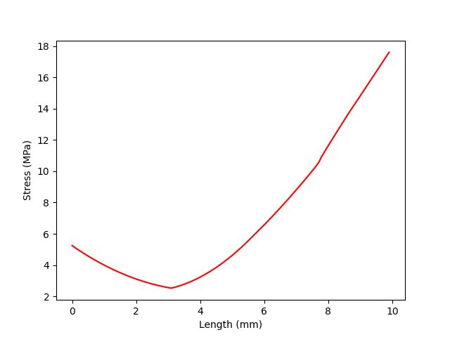
Create stress vs length chart.

x_initial = 0.0
length = [x_initial + delta * index for index in range(len(field_m.data))]
plt.plot(length, field_m.data, "r")
plt.xlabel("Length (%s)" % mesh.unit)
plt.ylabel("Stress (%s)" % field_m.unit)
plt.show()

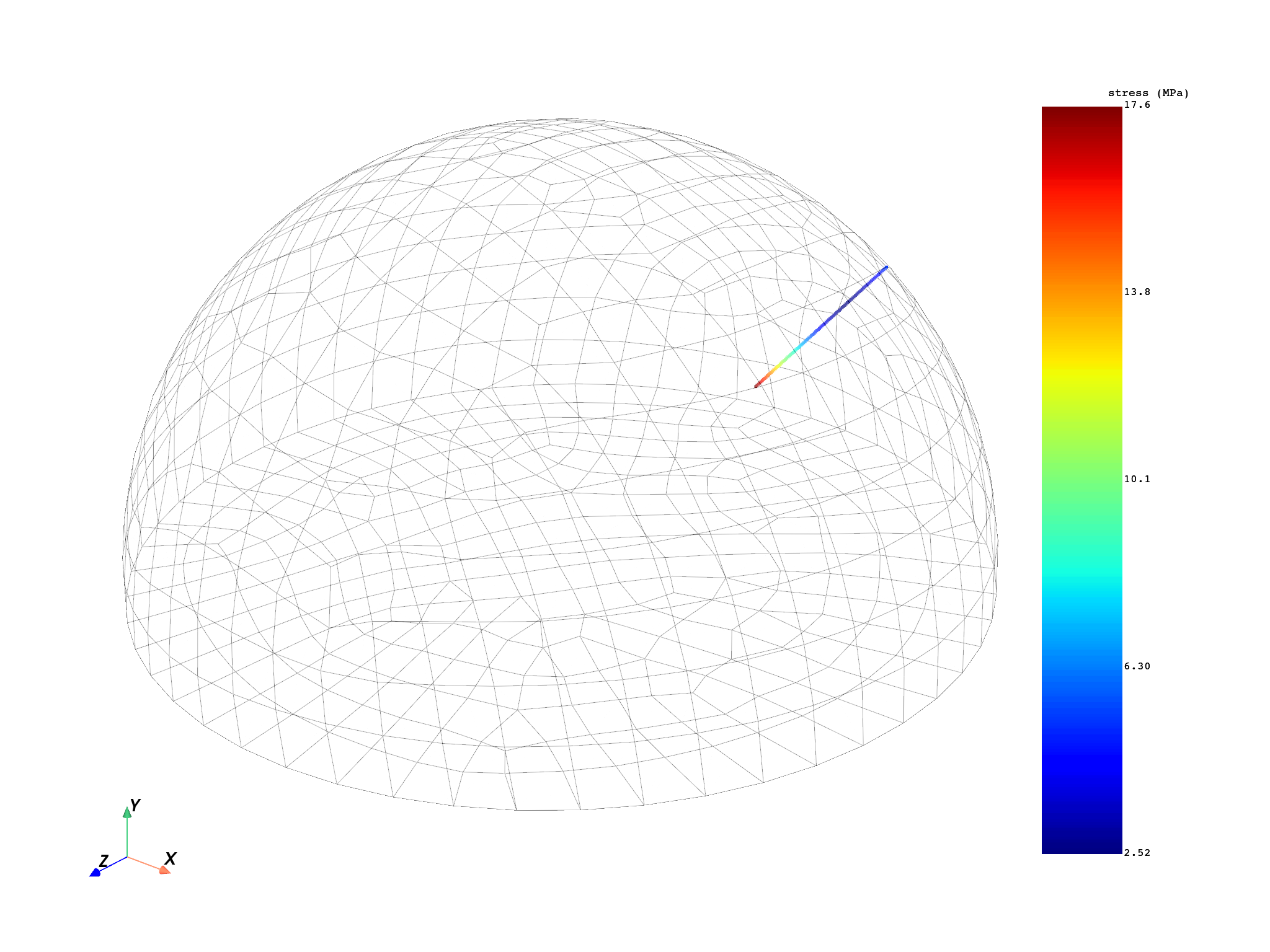
Create a plot to add both meshes, mesh_m (the mapped mesh) and mesh (the original mesh)

pl = DpfPlotter()
pl.add_field(field_m, mesh_m)
pl.add_mesh(mesh, style="surface", show_edges=True, color="w", opacity=0.3)
pl.show_figure(
    show_axes=True,
    cpos=[(62.687, 50.119, 67.247), (5.135, 6.458, -0.355), (-0.286, 0.897, -0.336)],
)