Expand harmonic modal superposition with DPF

Different types of linear dynamics expansions are implemented in DPF. With modal superposition used in harmonic analysis, modal coefficients are multiplied by mode shapes (of a previous modal analysis) to analyse a structure under given boundary conditions in a range of frequencies. Doing this expansion “on demand” in DPF instead of in the solver reduces the size of the result files.

from ansys.dpf import core as dpf
from ansys.dpf.core import examples

Create data sources

Create data sources with the mode shapes and the modal response. The expansion is recursive in DPF: first the modal response is read. Then, “upstream” mode shapes are found in the data sources, where they are read and expanded (mode shapes x modal response)

msup_files = examples.download_msup_files_to_dict()
data_sources = dpf.DataSources(msup_files["rfrq"])
up_stream_data_sources = dpf.DataSources(msup_files["mode"])
up_stream_data_sources.add_file_path(msup_files["rst"])

data_sources.add_upstream(up_stream_data_sources)

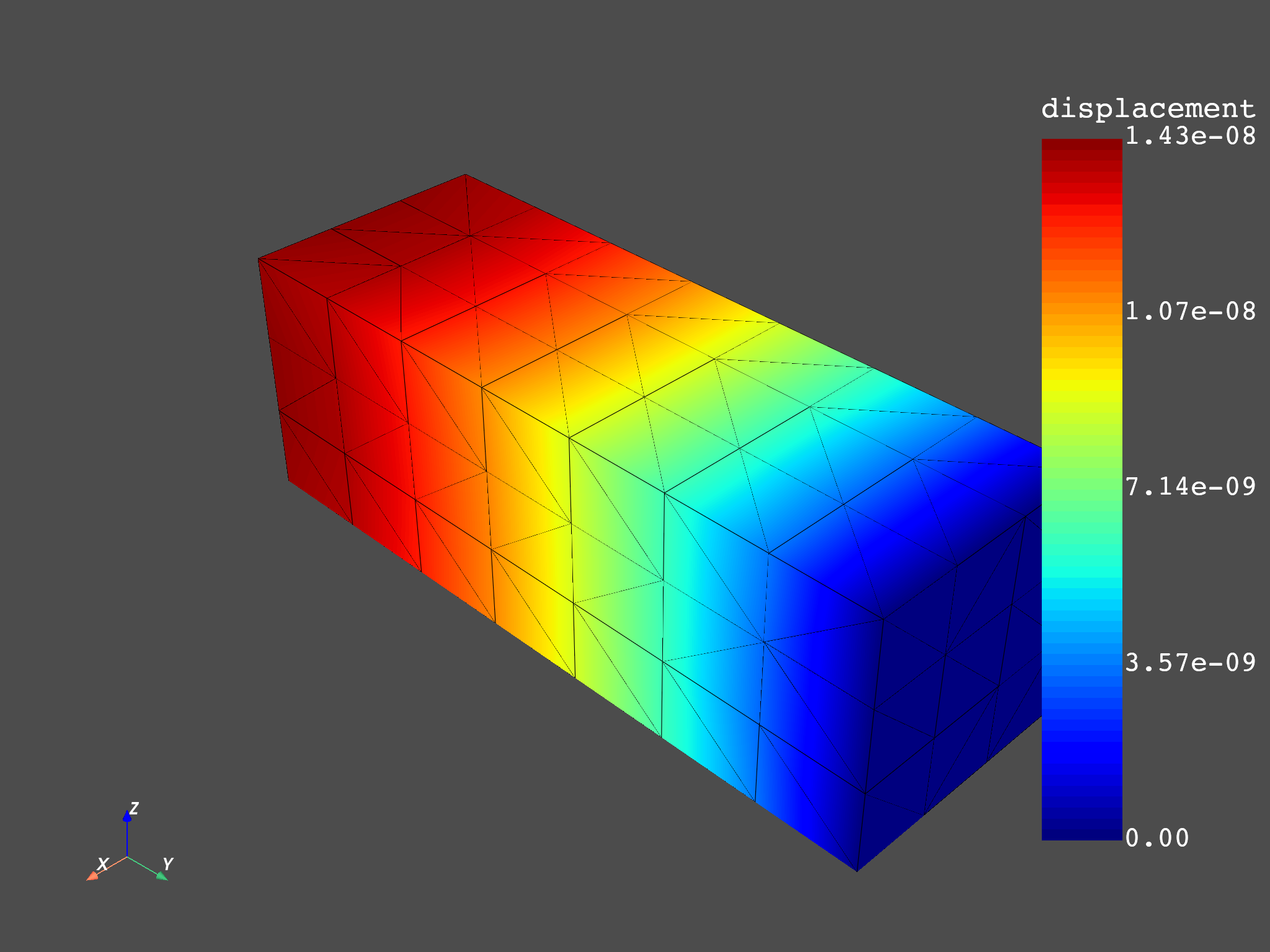
Compute displacements

Once the add_upstream() method puts the recursivity in the data sources, in a harmonic, transient, or modal analysis, computing displacements with or without expansion has the exact same syntax.

model = dpf.Model(data_sources)
disp = model.results.displacement.on_all_time_freqs.eval()

freq_scoping = disp.get_time_scoping()
for freq_set in freq_scoping:
    model.metadata.meshed_region.plot(disp.get_field_by_time_complex_ids(freq_set, 0))

• 
• 
• 
• 
• 
• 
• 
• 
• 
•