Compute iso-surfaces on fluid models

This example demonstrates how to compute iso-surfaces on fluid models.

Note

This example requires DPF 7.0 (ansys-dpf-server-2024-1-pre0) or above. For more information, see Compatibility.

Import the dpf-core module and its examples files.

import ansys.dpf.core as dpf
from ansys.dpf.core import examples
from ansys.dpf.core.plotter import DpfPlotter

Specify the file path.

We work on a cas/dat.h5 file with only nodal variables.

path = examples.download_cfx_heating_coil()
ds = dpf.DataSources()
ds.set_result_file_path(path["cas"], "cas")
ds.add_file_path(path["dat"], "dat")
streams = dpf.operators.metadata.streams_provider(data_sources=ds)

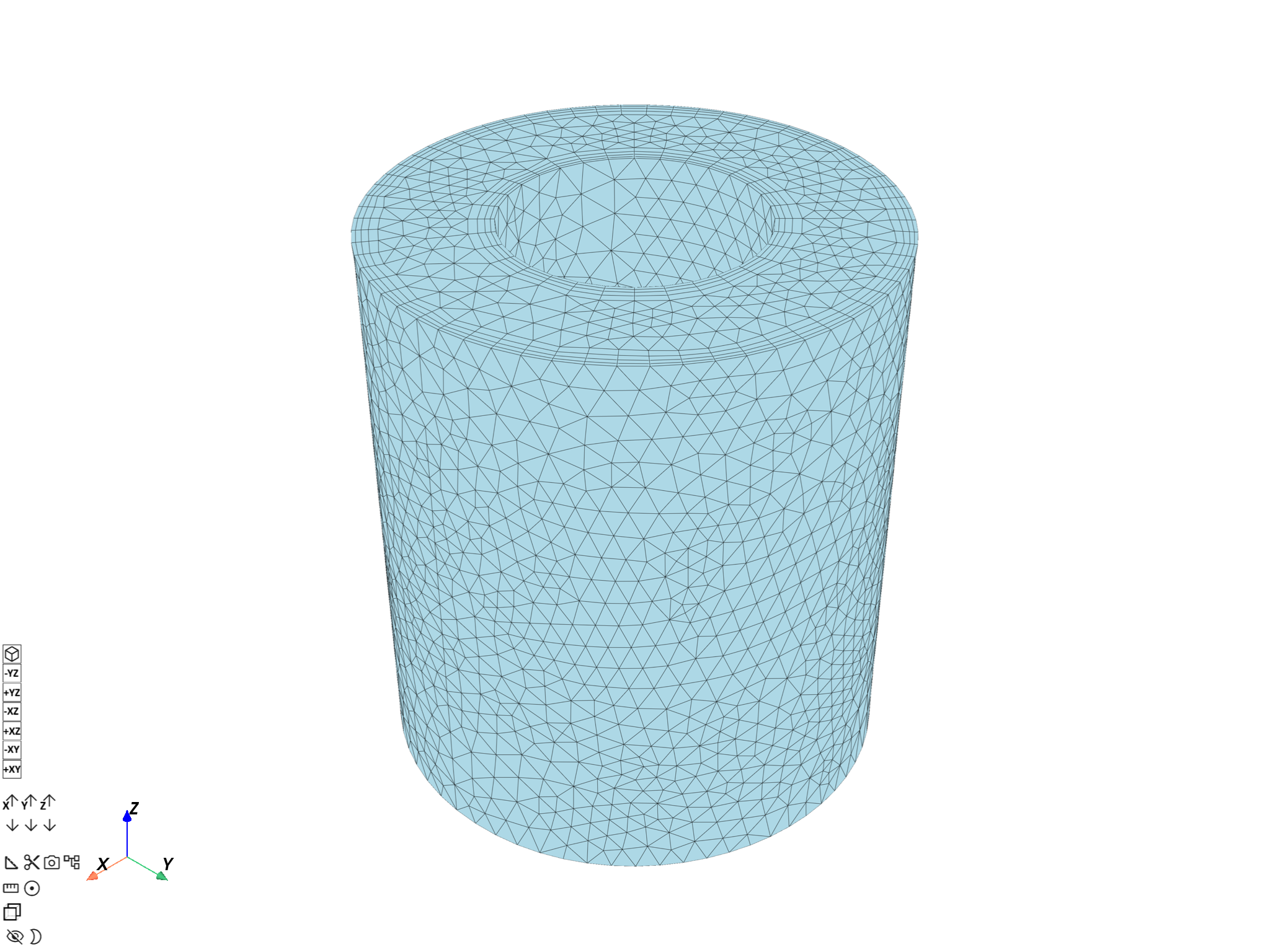
Whole mesh scoping.

We evaluate the mesh with the mesh_provider operator to scope the mesh_cut operator with the whole mesh.

whole_mesh = dpf.operators.mesh.mesh_provider(streams_container=streams).eval()
print(whole_mesh)

whole_mesh.plot()

DPF  Meshed Region:
  25456 nodes
  74882 elements
  Unit: m
  With solid (3D) elements

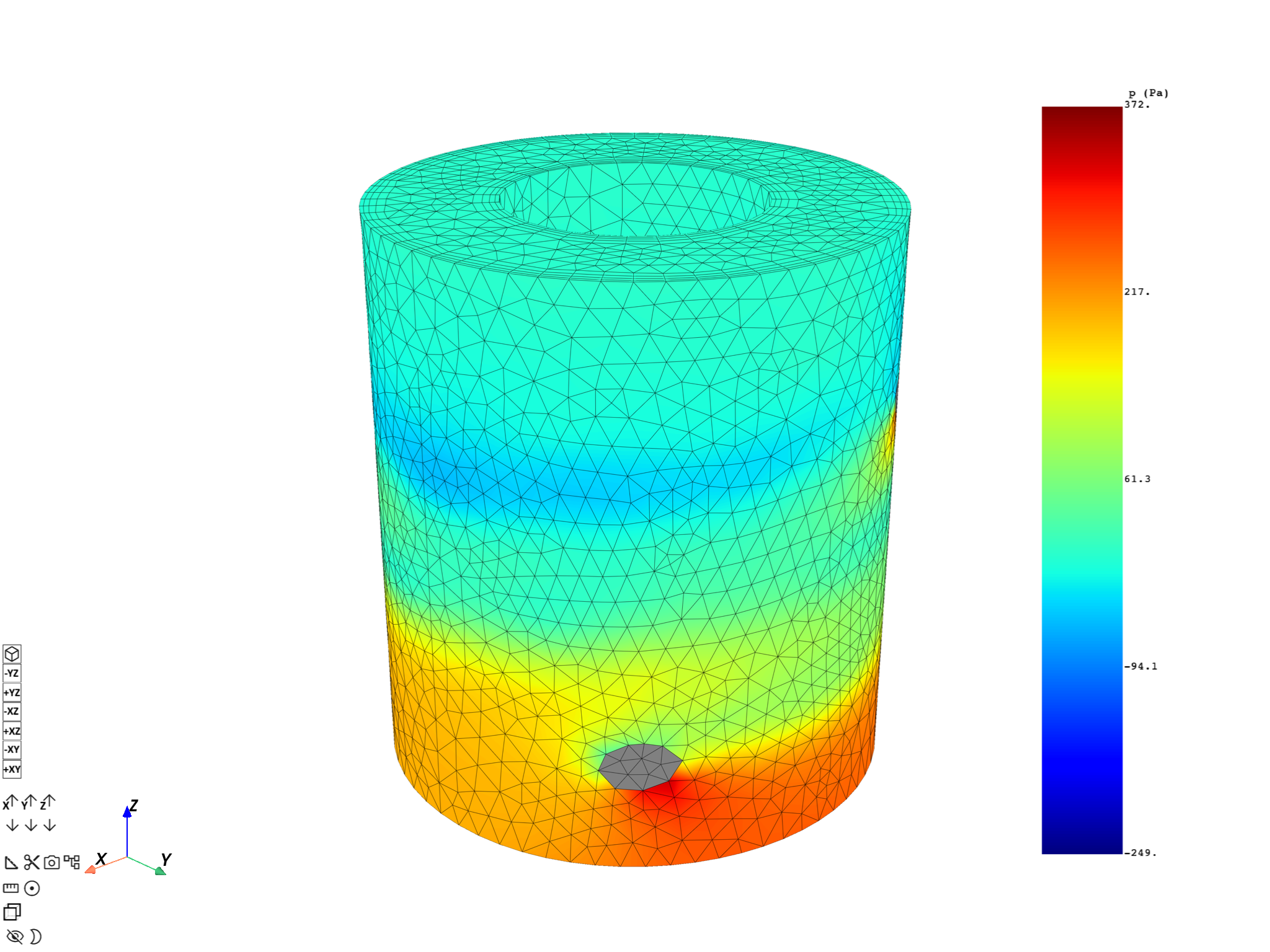
Extract the physics variable

Here we choose to work with the static pressure by default which is a scalar and nodal variable without multi-species/phases. With a multi-species case, select one using qualifier ellipsis pins and connecting a LabelSpace “species”/”phase”.

P_S = dpf.operators.result.static_pressure(streams_container=streams, mesh=whole_mesh).eval()
print(P_S[0])

pl = DpfPlotter()
pl.add_field(P_S[0])
cpos_mesh_variable = [
    (4.256160478475664, 4.73662111240005, 4.00410065817644),
    (-0.0011924505233764648, 1.8596649169921875e-05, 1.125),
    (-0.2738679385987956, -0.30771426079547065, 0.9112125360807675),
]
pl.show_figure(cpos=cpos_mesh_variable, show_axes=True)

DPF p_<Mixture> Field
  Location: Nodal
  Unit: Pa
  23648 entities
  Data: 1 components and 23648 elementary data

  Nodal
  IDs                   data(Pa)
  ------------          ----------
  1                     6.804220e+01

  2                     -1.422350e+01

  3                     2.180406e+02

  ...

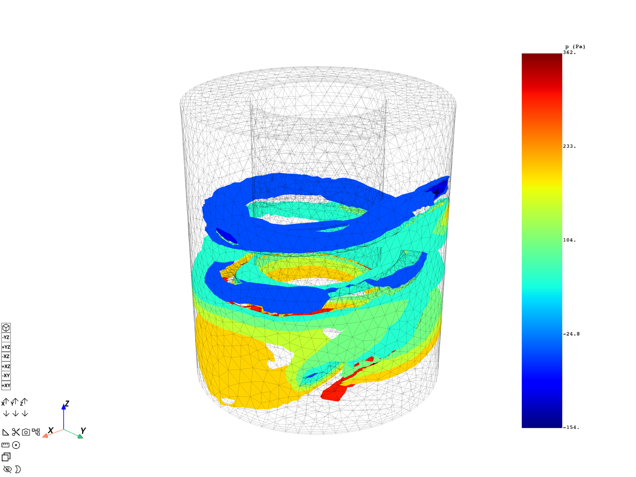
Evaluate iso-surfaces

We can finally use the iso_surfaces operator on this specific variable. We choose to cut the whole mesh with 9 iso-surface manually selected between the min and max of the static_pressure variable.

pl = DpfPlotter()
c_pos_iso = [
    (4.256160478475664, 4.73662111240005, 4.00410065817644),
    (-0.0011924505233764648, 1.8596649169921875e-05, 1.125),
    (-0.2738679385987956, -0.30771426079547065, 0.9112125360807675),
]
pl.add_mesh(
    meshed_region=whole_mesh,
    style="wireframe",
    show_edges=True,
    show_axes=True,
    color="black",
    opacity=0.3,
)

vec_iso_values = [-153.6, -100.0, -50.0, 50.0, 100.0, 150.0, 200.0, 300.0, 361.8]

iso_surfaces_op = dpf.operators.mesh.iso_surfaces(field=P_S[0], mesh=whole_mesh, slice_surfaces=True,
                                              vector_iso_values=vec_iso_values)

iso_surfaces_meshes = iso_surfaces_op.outputs.meshes()

iso_surfaces_fields = iso_surfaces_op.outputs.fields_container()

for i in range(len(iso_surfaces_fields)):
    pl.add_field(
        field=iso_surfaces_fields[i], meshed_region=iso_surfaces_meshes[i], style="surface", show_edges=False,
        show_axes=True
    )

pl.show_figure(show_axes=True, cpos=c_pos_iso)

Important note

Iso-surfaces computation through the mesh_cut operator are only supported for Nodal Fields. For Elemental variables, you must perform an averaging operation on the Nodes before running the mesh_cut operator. This can be done by chaining the elemental_to_nodal operator output with the mesh_cut operator input.