Expand mesh and results for modal cyclic symmetry

This example shows a modal cyclic symmetry model with mesh and results expansions.

from ansys.dpf import core as dpf
from ansys.dpf.core import examples

Create the model and display the state of the result.

model = dpf.Model(examples.find_simple_cyclic())
print(model)

DPF Model
------------------------------
Modal analysis
Unit system: MKS: m, kg, N, s, V, A, degC
Physics Type: Mechanical
Available results:
     -  displacement: Nodal Displacement
     -  stress: ElementalNodal Stress
     -  elemental_volume: Elemental Volume
     -  stiffness_matrix_energy: Elemental Energy-stiffness matrix
     -  artificial_hourglass_energy: Elemental Hourglass Energy
     -  kinetic_energy: Elemental Kinetic Energy
     -  co_energy: Elemental co-energy
     -  incremental_energy: Elemental incremental energy
     -  thermal_dissipation_energy: Elemental thermal dissipation energy
     -  element_orientations: ElementalNodal Element Euler Angles
     -  structural_temperature: ElementalNodal Structural temperature
------------------------------
DPF  Meshed Region:
  51 nodes
  4 elements
  Unit: m
  With solid (3D) elements
------------------------------
DPF  Time/Freq Support:
  Number of sets: 30
Cumulative     Frequency (Hz) LoadStep       Substep        Harmonic index
1              670386,325235  1              1              0,000000
2              872361,424038  1              2              0,000000
3              1142526,525324 1              3              0,000000
4              1252446,741551 1              4              0,000000
5              1257379,552140 1              5              0,000000
6              1347919,358013 1              6              0,000000
7              679667,393214  2              1              1,000000
8              679667,393214  2              2              -1,000000
9              899321,218481  2              3              -1,000000
10             899321,218481  2              4              1,000000
11             1128387,049511 2              5              1,000000
12             1128387,049511 2              6              -1,000000
13             708505,071361  3              1              -2,000000
14             708505,071361  3              2              2,000000
15             966346,820117  3              3              2,000000
16             966346,820117  3              4              -2,000000
17             1031249,070606 3              5              -2,000000
18             1031249,070606 3              6              2,000000
19             757366,624982  4              1              -3,000000
20             757366,624982  4              2              3,000000
21             926631,623058  4              3              -3,000000
22             926631,623058  4              4              3,000000
23             1035144,649248 4              5              3,000000
24             1035144,649248 4              6              -3,000000
25             807882,379030  5              1              4,000000
26             856868,410638  5              2              4,000000
27             1063247,283632 5              3              4,000000
28             1185511,741334 5              4              4,000000
29             1278969,844256 5              5              4,000000
30             1355579,879820 5              6              4,000000

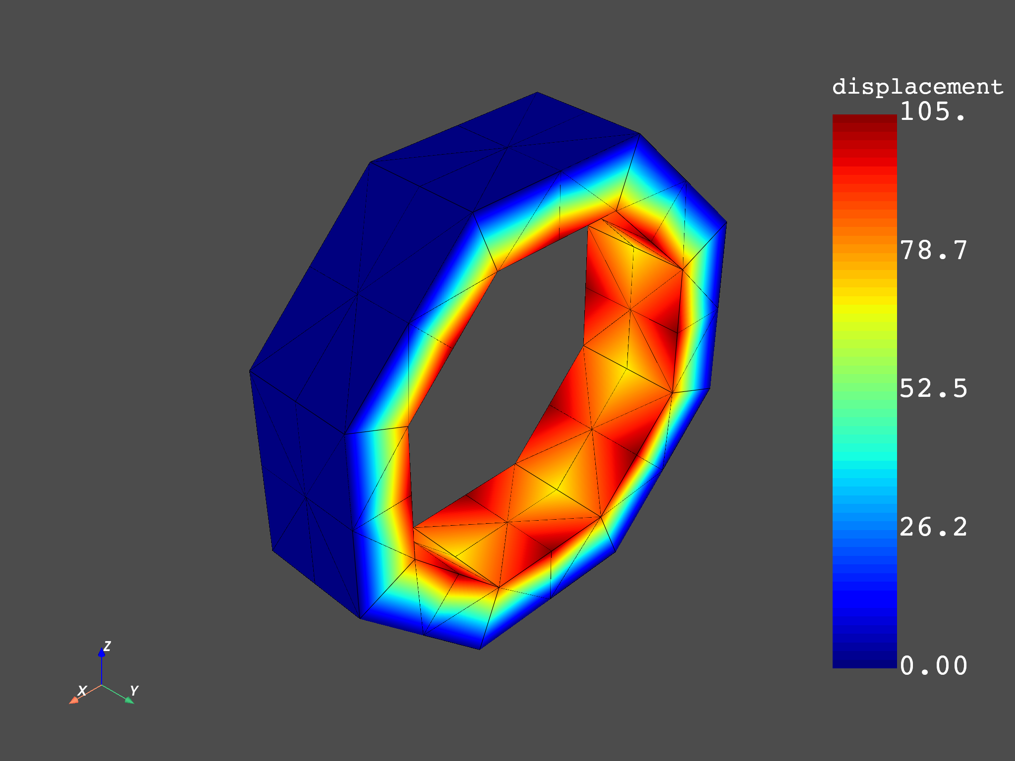
Expand displacement results

This example expands displacement results, by default on all nodes and the first time step. Note that the displacements are expanded using the read_cyclic property with 2 as an argument (1 does not perform expansion of the cyclic symmetry).

# Create displacement cyclic operator
u_cyc = model.results.displacement()
u_cyc.inputs.read_cyclic(2)

# expand the displacements
fields = u_cyc.outputs.fields_container()

# # get the expanded mesh
mesh_provider = model.metadata.mesh_provider
mesh_provider.inputs.read_cyclic(2)
mesh = mesh_provider.outputs.mesh()

# plot the expanded result on the expanded mesh
mesh.plot(fields[0])

(None, <pyvista.plotting.plotter.Plotter object at 0x00000225F9850440>)

Expand stresses at a given time step

# define stress expansion operator and request stresses at time set = 8
scyc_op = model.results.stress()
scyc_op.inputs.read_cyclic(2)
scyc_op.inputs.time_scoping.connect([8])

# request the results averaged on the nodes
scyc_op.inputs.requested_location.connect(dpf.locations.nodal)

# request equivalent von mises operator and connect it to stress operator
eqv = dpf.operators.invariant.von_mises_eqv_fc(scyc_op)

# expand the results and get stress eqv
fields = eqv.outputs.fields_container()

# plot the expanded result on the expanded mesh
# mesh.plot(fields[0])

Expand stresses at given sectors

# define stress expansion operator and request stresses at time set = 8
# request the results averaged on the nodes
# request results on sectors 1, 3 and 5
scyc_op = dpf.operators.result.stress(
    streams_container=model.metadata.streams_provider,
    time_scoping=[8],
    requested_location=dpf.locations.nodal,
    sectors_to_expand=[1, 3, 5],
    read_cyclic=2,
)

# extract Sx (use component selector and select the first component)
comp_sel = dpf.operators.logic.component_selector_fc(scyc_op, 0)

# expand the displacements and get the results
fields = comp_sel.outputs.fields_container()

# plot the expanded result on the expanded mesh
# mesh.plot(fields[0])

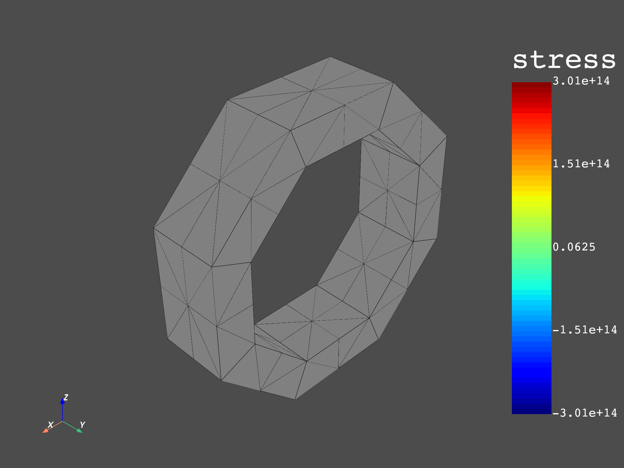
Expand stresses and average to elemental location

# define stress expansion operator and request stresses at time set = 8
scyc_op = dpf.operators.result.stress(
    streams_container=model.metadata.streams_provider,
    time_scoping=[8],
    sectors_to_expand=[1, 3, 5],
    bool_rotate_to_global=False,
    read_cyclic=2,
)

# request to elemental averaging operator
to_elemental = dpf.operators.averaging.to_elemental_fc(scyc_op)

# extract Sy (use component selector and select the component 1)
comp_sel = dpf.operators.logic.component_selector_fc(to_elemental, 1)

# expand the displacements and get the results
fields = comp_sel.outputs.fields_container()

# # plot the expanded result on the expanded mesh
mesh.plot(fields)

(None, <pyvista.plotting.plotter.Plotter object at 0x00000225F9B45490>)