Working with a result file

This example shows how to write and upload files on the server machine and then download them back on the client side. The resulting fields container is then exported to a CSV file.

Load a model from the DPF-Core examples: ansys.dpf.core module.

from ansys.dpf import core as dpf
from ansys.dpf.core import examples

model = dpf.Model(examples.find_simple_bar())
mesh = model.metadata.meshed_region

Get and plot the fields container for the result

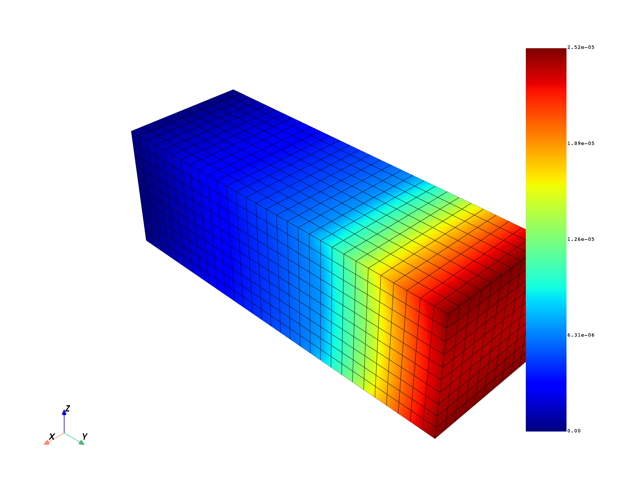
Get the fields container for the result and plot it so you can compare it later:

displacement_operator = model.results.displacement()
fc_out = displacement_operator.outputs.fields_container()
mesh.plot(fc_out)

Export result

Export the fields container in the CSV format:

from pathlib import Path

csv_file_name = "simple_bar_fc.csv"
# Define an output path for the resulting .csv file
if not dpf.SERVER.local_server:
    # Define it server-side if using a remote server
    tmp_dir_path = dpf.core.make_tmp_dir_server(dpf.SERVER)
    server_file_path = Path(dpf.path_utilities.join(tmp_dir_path, csv_file_name))
else:
    server_file_path = Path.cwd() / csv_file_name

# Perform the export to csv on the server side
export_csv_operator = dpf.operators.serialization.field_to_csv()
export_csv_operator.inputs.field_or_fields_container.connect(fc_out)
export_csv_operator.inputs.file_path.connect(server_file_path)
export_csv_operator.run()

Download CSV result file

Download the file simple_bar_fc.csv:

if not dpf.SERVER.local_server:
    downloaded_client_file_path = Path.cwd() / "simple_bar_fc_downloaded.csv"
    dpf.download_file(server_file_path, downloaded_client_file_path)
else:
    downloaded_client_file_path = server_file_path

Load CSV result file as operator input

Load the fields container contained in the CSV file as an operator input:

my_data_sources = dpf.DataSources(server_file_path)
import_csv_operator = dpf.operators.serialization.csv_to_field()
import_csv_operator.inputs.data_sources.connect(my_data_sources)
server_fc_out = import_csv_operator.outputs.fields_container()
mesh.plot(server_fc_out)

# Remove file to avoid polluting.
downloaded_client_file_path.unlink()

Make operations over the fields container

Use this fields container to get the minimum displacement:

min_max_op = dpf.operators.min_max.min_max_fc()
min_max_op.inputs.fields_container.connect(server_fc_out)
min_field = min_max_op.outputs.field_min()
min_field.data

DPFArray([[-8.202171e-07, -6.265107e-06, -2.444680e-05]])

Compare the original and the new fields container

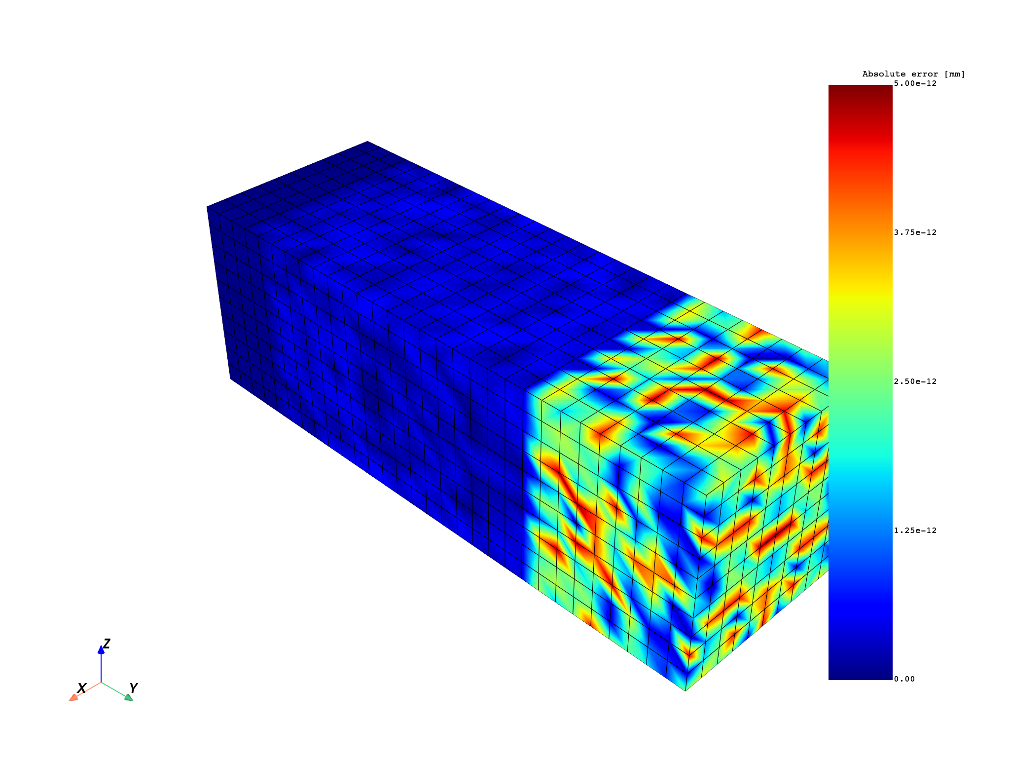
Subtract the two fields and plot an error map:

abs_error = (fc_out - server_fc_out).eval()

divide = dpf.operators.math.component_wise_divide()
divide.inputs.fieldA.connect(fc_out - server_fc_out)
divide.inputs.fieldB.connect(fc_out)
scale = dpf.operators.math.scale()
scale.inputs.field.connect(divide)
scale.inputs.weights.connect(100.0)
rel_error = scale.eval()

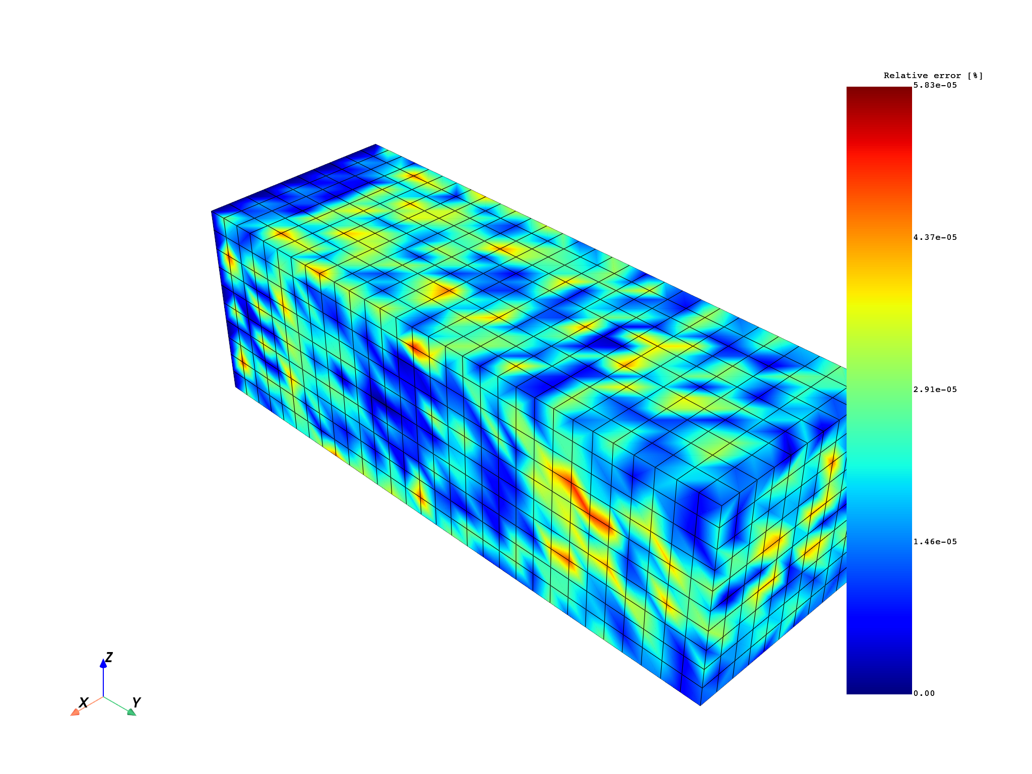
Plot both absolute and relative error fields

Note that the absolute error is bigger where the displacements are bigger, at the tip of the geometry. Instead, the relative error is similar across the geometry since we are dividing by the displacements fc_out. Both plots show errors that can be understood as zero due to machine precision (1e-12 mm for the absolute error and 1e-5% for the relative error).

mesh.plot(abs_error, scalar_bar_args={"title": "Absolute error [mm]"})
mesh.plot(rel_error, scalar_bar_args={"title": "Relative error [%]"})

• 
•