Processing data basics

Data Processing consists in a series of operations applied to data to achieve a goal. DPF enables you to access and transform simulation data using customizable workflows.

There is an extensive catalog of operators with different kinds and complexity that can be used together.

The tutorials in this section presents a basic application of PyDPF-Core as post-processing tool.

Postprocessing main steps

There are four main steps to transform simulation data into output data that can be used to visualize and analyze simulation results:

1

Importing and opening results files

1- Import and open results files

2

Access and extract results

2- Access and extract results

3

Transform available data

3- Transform available data

4

Visualize the data

4- Visualize the data

Download tutorial as Python script Download tutorial as Jupyter notebook

1- Import and open results files

First, import the DPF-Core module as dpf and import the included examples file

# Import the ansys.dpf.core module as ``dpf``
from ansys.dpf import core as dpf
# Import the examples module
from ansys.dpf.core import examples
# Import the operators module
from ansys.dpf.core import operators as ops

`DataSources’ is a class that manages paths to their files. Use this object to declare data inputs for DPF and define their locations.

# Define the DataSources object
my_data_sources = dpf.DataSources(result_path=examples.find_simple_bar())

The Model class creates and evaluates common readers for the files it is given, such as a mesh provider, a result info provider, and a streams provider. It provides dynamically built methods to extract the results available in the files, as well as many shortcuts to facilitate exploration of the available data.

Printing the model displays:

• Analysis type

• Available results

• Size of the mesh

• Number of results

# Define the Model object
my_model = dpf.Model(data_sources=my_data_sources)
print(my_model)

DPF Model
------------------------------
Static analysis
Unit system: MKS: m, kg, N, s, V, A, degC
Physics Type: Mechanical
Available results:
     -  displacement: Nodal Displacement
     -  element_nodal_forces: ElementalNodal Element nodal Forces
     -  elemental_volume: Elemental Volume
     -  stiffness_matrix_energy: Elemental Energy-stiffness matrix
     -  artificial_hourglass_energy: Elemental Hourglass Energy
     -  kinetic_energy: Elemental Kinetic Energy
     -  co_energy: Elemental co-energy
     -  incremental_energy: Elemental incremental energy
     -  thermal_dissipation_energy: Elemental thermal dissipation energy
     -  element_orientations: ElementalNodal Element Euler Angles
     -  structural_temperature: ElementalNodal Structural temperature
------------------------------
DPF  Meshed Region: 
  3751 nodes 
  3000 elements 
  Unit: m 
  With solid (3D) elements
------------------------------
DPF  Time/Freq Support: 
  Number of sets: 1 
Cumulative     Time (s)       LoadStep       Substep         
1              1.000000       1              1               

2- Access and extract results

We see in the model that a displacement result is available. You can access this result by:

# Define the displacement results through the models property `results`
my_displacements = my_model.results.displacement.eval()
print(my_displacements)

DPF displacement(s)Fields Container
  with 1 field(s)
  defined on labels: time 

  with:
  - field 0 {time:  1} with Nodal location, 3 components and 3751 entities.

The displacement data can be extract by:

# Extract the data of the displacement field
my_displacements_0 = my_displacements[0].data
print(my_displacements_0)

[[-1.22753781e-08 -1.20861254e-06 -5.02681396e-06]
 [-9.46666013e-09 -1.19379712e-06 -4.64249826e-06]
 [-1.22188426e-08 -1.19494216e-06 -4.63117832e-06]
 ...
 [-1.35911608e-08  1.52559428e-06 -4.29246409e-06]
 [-1.91212290e-08  1.52577102e-06 -4.28782940e-06]
 [-2.69632909e-08  1.52485289e-06 -4.27831232e-06]]

3- Transform available data

Several transformations can be made with the data. They can be a single operation, by using only one operator, or they can represent a succession of operations, by defining a workflow with chained operators.

Here we star by computing the displacements norm.

# Define the norm operator (here for a fields container) for the displacement
my_norm = ops.math.norm_fc(fields_container=my_displacements).eval()
print(my_norm[0].data)

[5.17008254e-06 4.79354058e-06 4.78287034e-06 ... 4.55553187e-06
 4.55124420e-06 4.54201053e-06]

Then we compute the maximum values of the normalised displacement

# Define the maximum operator and chain it to the norm operator
my_max= ops.min_max.min_max_fc(fields_container=my_norm).outputs.field_max()
print(my_max)

DPF displacement_1.s Field
  Location: Nodal
  Unit: m
  1 entities 
  Data: 1 components and 1 elementary data 

  IDs                   data(m)
  ------------          ----------
  0                     2.523683e-05   
                        

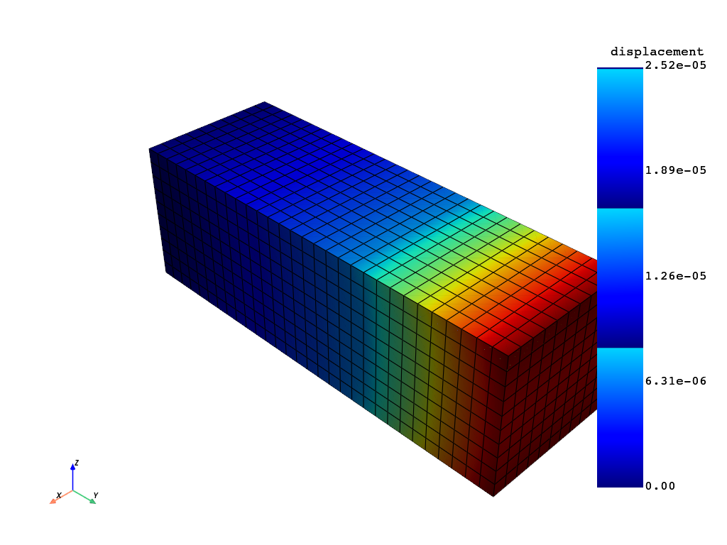
4- Visualize the data

Plot the transformed displacement results

# Define the support of the plot (here we plot the displacement over the mesh)
my_model.metadata.meshed_region.plot(field_or_fields_container=my_displacements)

(None, <pyvista.plotting.plotter.Plotter at 0x14b34850110>)