Animate data over time

MAPDL LS-DYNA FLUENT CFX

This tutorial demonstrates how to create 3D animations of data in time.

To animate data across time, the data must be stored in a FieldsContainer with a time label.

Get the result files

For this tutorial, we use a case available in the examples module. For more information about how to import your own result file in DPF, see the Import Data tutorial section.

from ansys.dpf import core as dpf
from ansys.dpf.core import examples, operators as ops

result_file_path = examples.find_msup_transient()
model = dpf.Model(data_sources=result_file_path)

Define a time scoping

To animate across time, define the time steps of interest. This tutorial retrieves all time steps available in TimeFreqSupport, but you can also filter them. For more information on how to define a scoping, see the narrow_down_data tutorial in the Import Data section.

time_steps = model.metadata.time_freq_support.time_frequencies

Extract the results

Extract the results to animate. In this tutorial, we extract displacement and stress results.

Note

Only the elemental, nodal, or faces locations are supported for animations. overall and elemental_nodal locations are not currently supported.

Get the displacement fields (already on nodes) at all time steps.

disp_fc = model.results.displacement(time_scoping=time_steps).eval()
print(disp_fc)

DPF  Fields Container
  with 20 field(s)
  defined on labels: time

  with:
  - field 0 {time:  1} with Nodal location, 3 components and 393 entities.
  - field 1 {time:  2} with Nodal location, 3 components and 393 entities.
  - field 2 {time:  3} with Nodal location, 3 components and 393 entities.
  - field 3 {time:  4} with Nodal location, 3 components and 393 entities.
  - field 4 {time:  5} with Nodal location, 3 components and 393 entities.
  - field 5 {time:  6} with Nodal location, 3 components and 393 entities.
  - field 6 {time:  7} with Nodal location, 3 components and 393 entities.
  - field 7 {time:  8} with Nodal location, 3 components and 393 entities.
  - field 8 {time:  9} with Nodal location, 3 components and 393 entities.
  - field 9 {time:  10} with Nodal location, 3 components and 393 entities.
  - field 10 {time:  11} with Nodal location, 3 components and 393 entities.
  - field 11 {time:  12} with Nodal location, 3 components and 393 entities.
  - field 12 {time:  13} with Nodal location, 3 components and 393 entities.
  - field 13 {time:  14} with Nodal location, 3 components and 393 entities.
  - field 14 {time:  15} with Nodal location, 3 components and 393 entities.
  - field 15 {time:  16} with Nodal location, 3 components and 393 entities.
  - field 16 {time:  17} with Nodal location, 3 components and 393 entities.
  - field 17 {time:  18} with Nodal location, 3 components and 393 entities.
  - field 18 {time:  19} with Nodal location, 3 components and 393 entities.
  - field 19 {time:  20} with Nodal location, 3 components and 393 entities.

Get the stress fields on nodes at all time steps. Request nodal location as the default elemental_nodal location is not supported for animations.

stress_fc = (
    model.results.stress.on_location(location=dpf.locations.nodal)
    .on_time_scoping(time_scoping=time_steps)
    .eval()
)
print(stress_fc)

DPF  Fields Container
  with 20 field(s)
  defined on labels: time

  with:
  - field 0 {time:  1} with Nodal location, 6 components and 393 entities.
  - field 1 {time:  2} with Nodal location, 6 components and 393 entities.
  - field 2 {time:  3} with Nodal location, 6 components and 393 entities.
  - field 3 {time:  4} with Nodal location, 6 components and 393 entities.
  - field 4 {time:  5} with Nodal location, 6 components and 393 entities.
  - field 5 {time:  6} with Nodal location, 6 components and 393 entities.
  - field 6 {time:  7} with Nodal location, 6 components and 393 entities.
  - field 7 {time:  8} with Nodal location, 6 components and 393 entities.
  - field 8 {time:  9} with Nodal location, 6 components and 393 entities.
  - field 9 {time:  10} with Nodal location, 6 components and 393 entities.
  - field 10 {time:  11} with Nodal location, 6 components and 393 entities.
  - field 11 {time:  12} with Nodal location, 6 components and 393 entities.
  - field 12 {time:  13} with Nodal location, 6 components and 393 entities.
  - field 13 {time:  14} with Nodal location, 6 components and 393 entities.
  - field 14 {time:  15} with Nodal location, 6 components and 393 entities.
  - field 15 {time:  16} with Nodal location, 6 components and 393 entities.
  - field 16 {time:  17} with Nodal location, 6 components and 393 entities.
  - field 17 {time:  18} with Nodal location, 6 components and 393 entities.
  - field 18 {time:  19} with Nodal location, 6 components and 393 entities.
  - field 19 {time:  20} with Nodal location, 6 components and 393 entities.

Animate the results

Animate the results with FieldsContainer.animate(). You can animate on a deformed mesh (color map + mesh deformation) or on a static mesh (color map only).

Default behavior of animate():

• Displays the norm of the data components.

• Displays data at the top layer for shells.

• Displays the deformed mesh when animating displacements.

• Displays the static mesh for other result types.

• Uses a constant uniform scale factor of 1.0 when deforming the mesh.

You can animate any result on a deformed geometry by providing displacement results in the deform_by parameter. It accepts a result object, an Operator (must evaluate to a FieldsContainer of the same length), or a FieldsContainer of the same length.

Note

The behavior of animate() is defined by a Workflow that it creates internally and feeds to an Animator. This workflow loops over a field of frame indices and for each frame generates a field of norm contours to render, as well as a displacement field to deform the mesh if deform_by is provided.

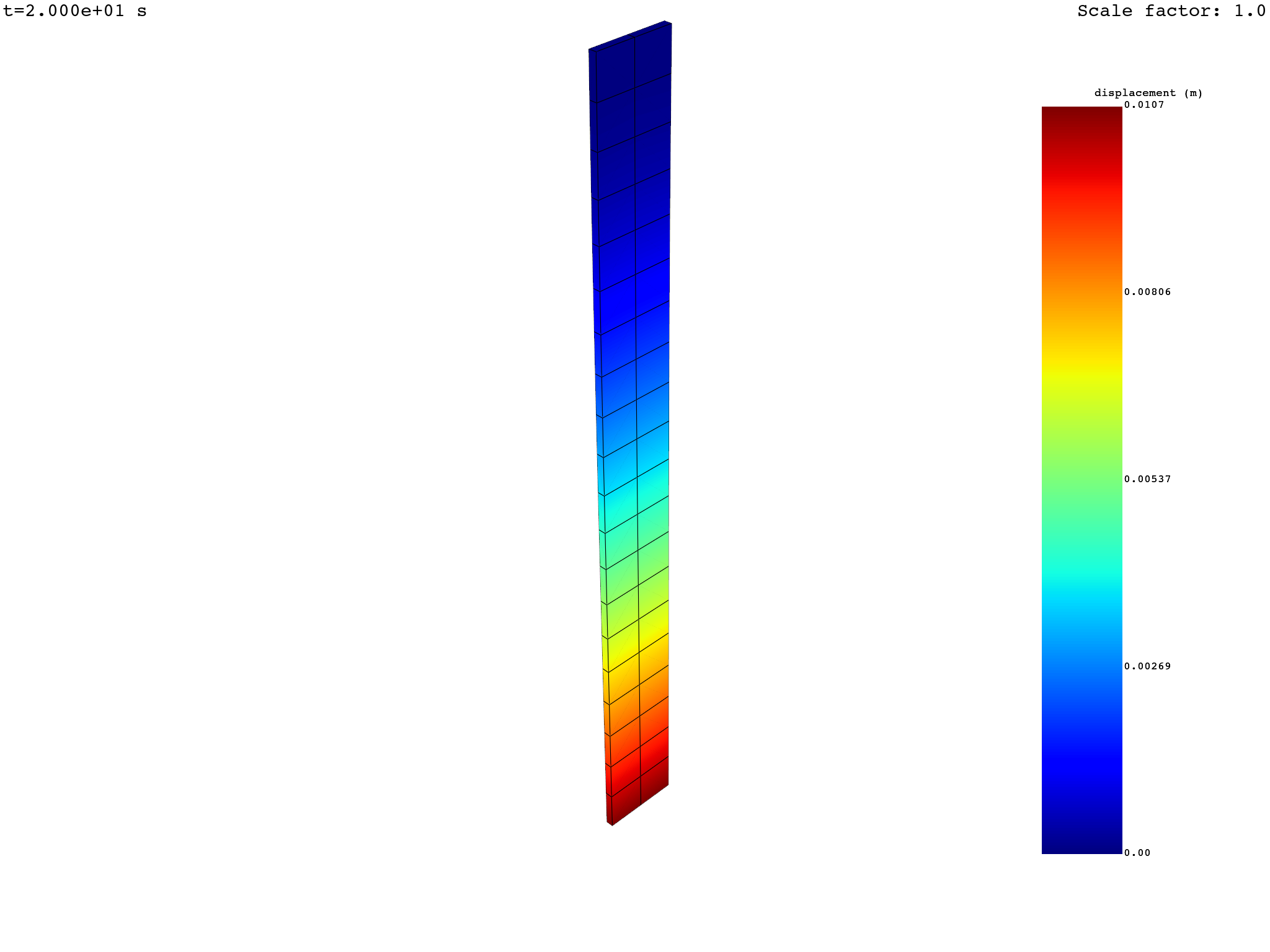
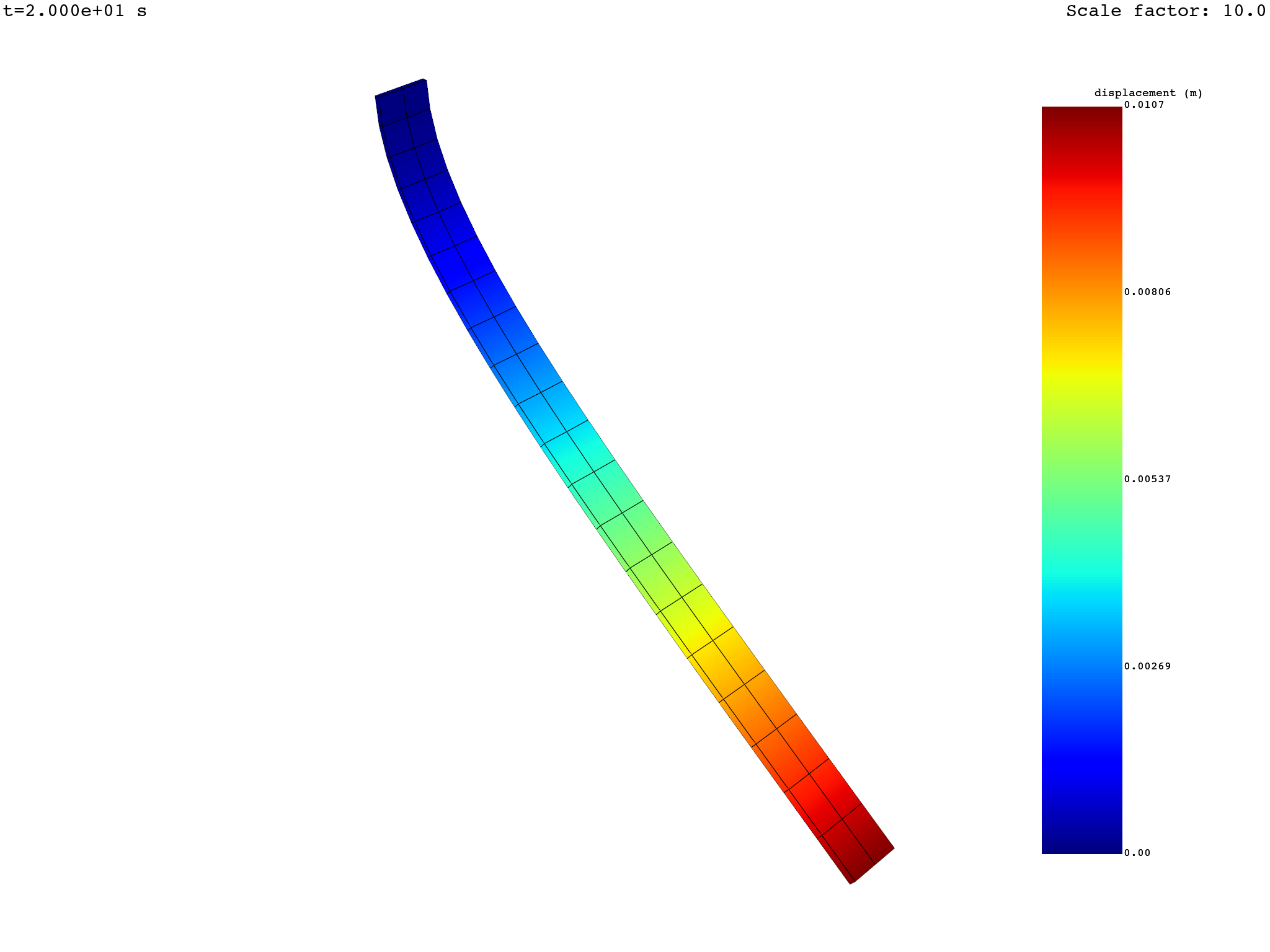
Animate the displacement results — deformed mesh

disp_fc.animate()

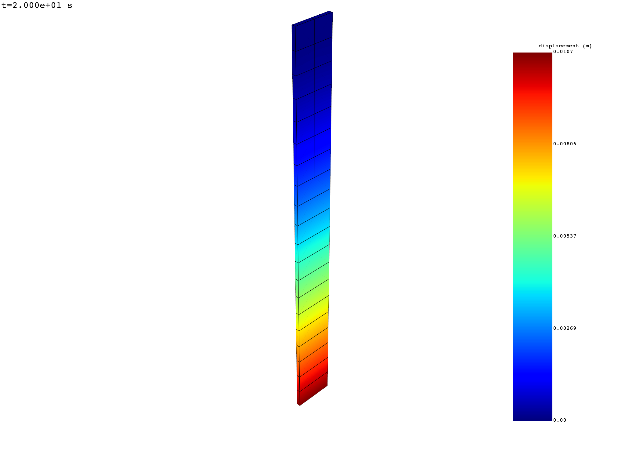
Animate the displacement results — static mesh

Use deform_by=False to animate on a static mesh.

disp_fc.animate(deform_by=False)

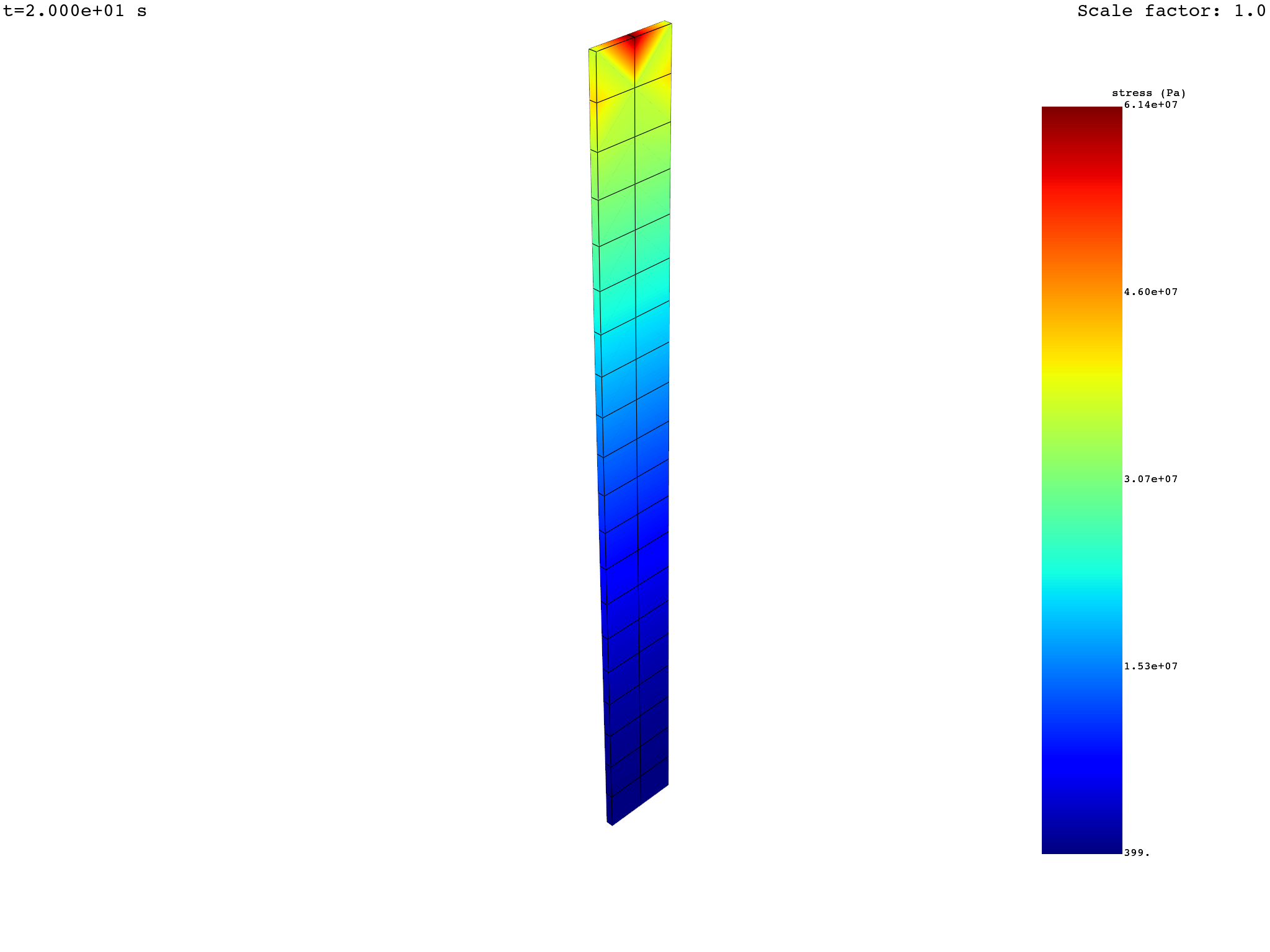
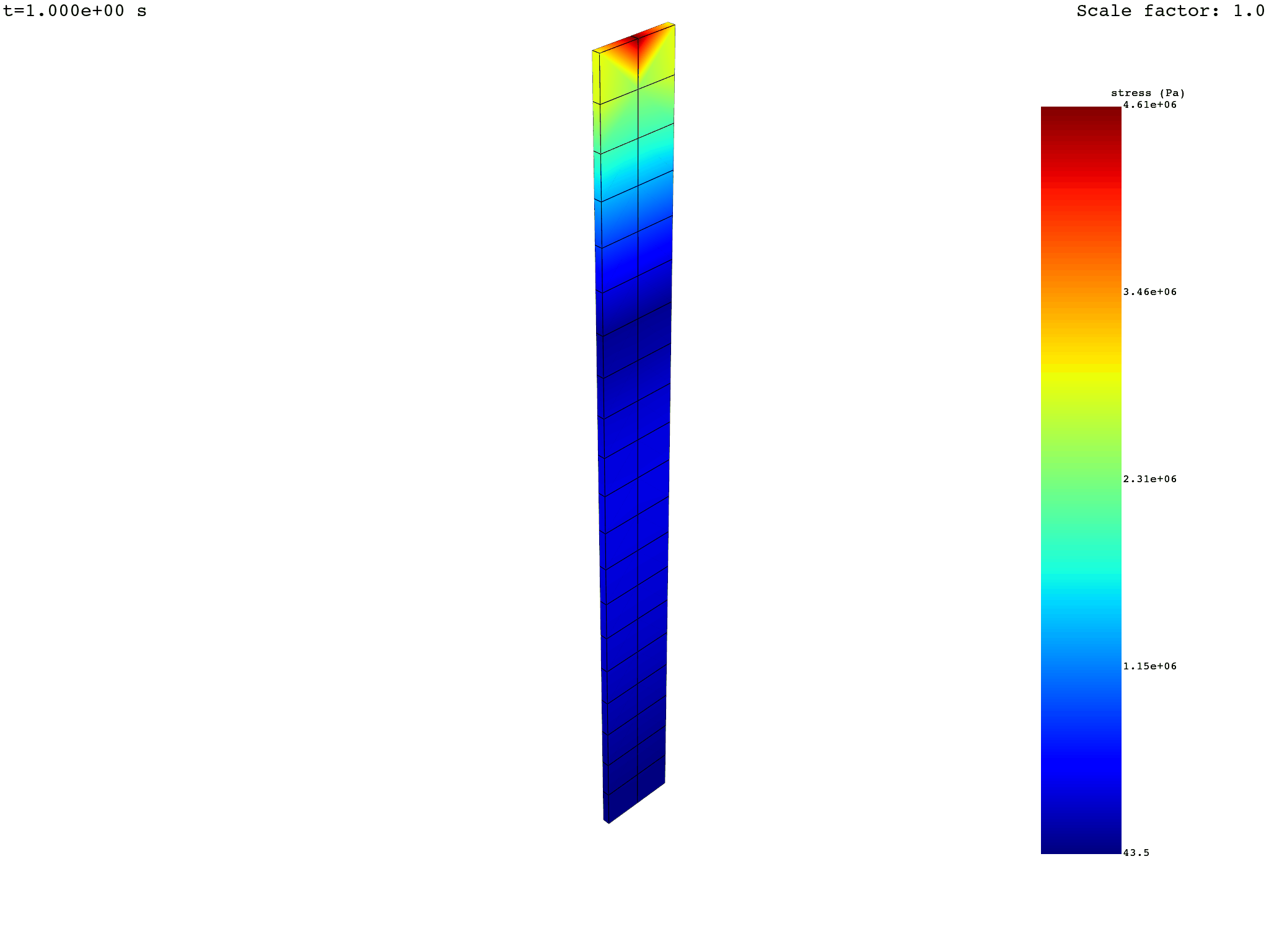
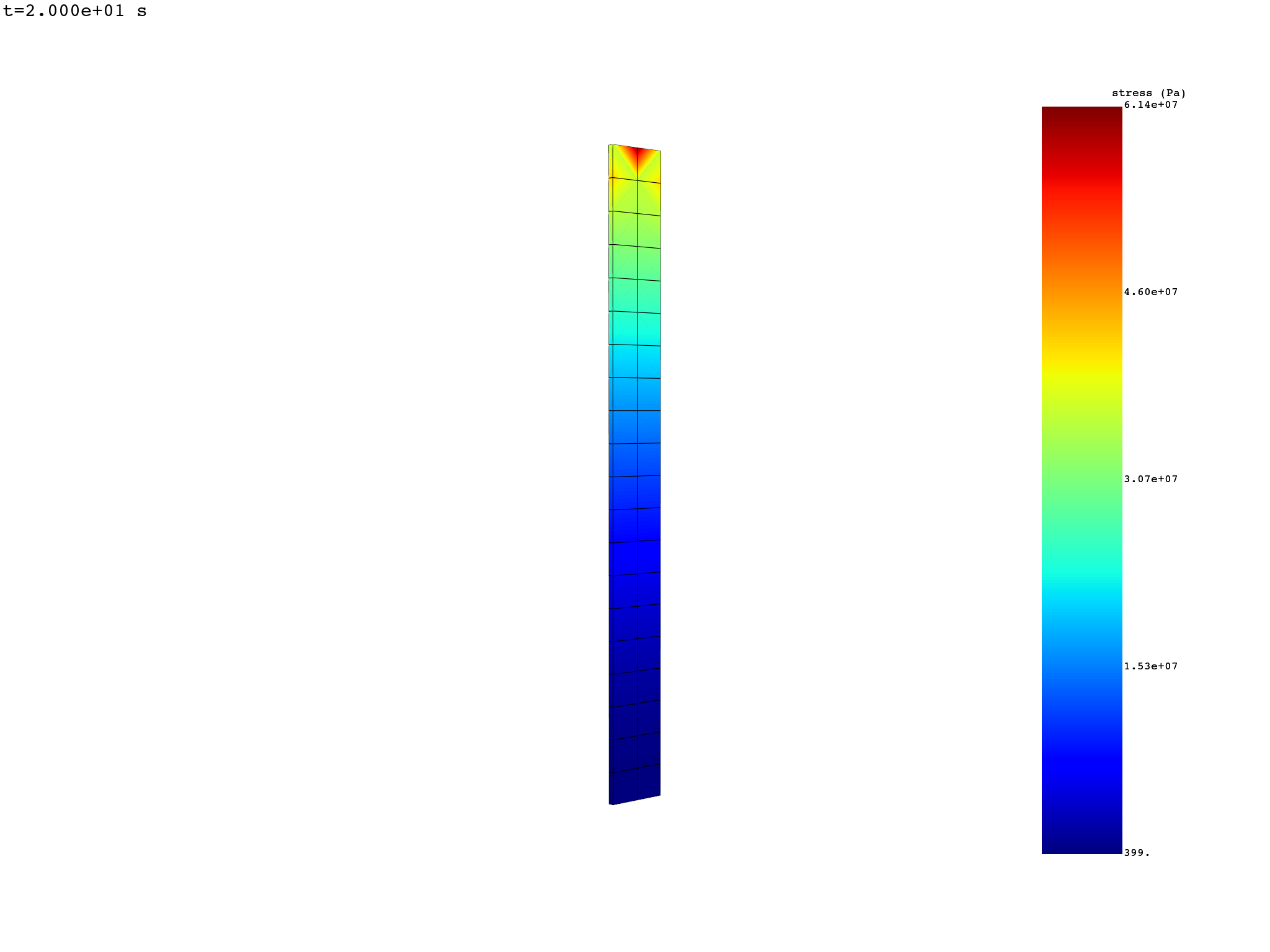
Animate the stress — deformed mesh

Pass the displacement FieldsContainer to deform_by.

stress_fc.animate(deform_by=disp_fc)

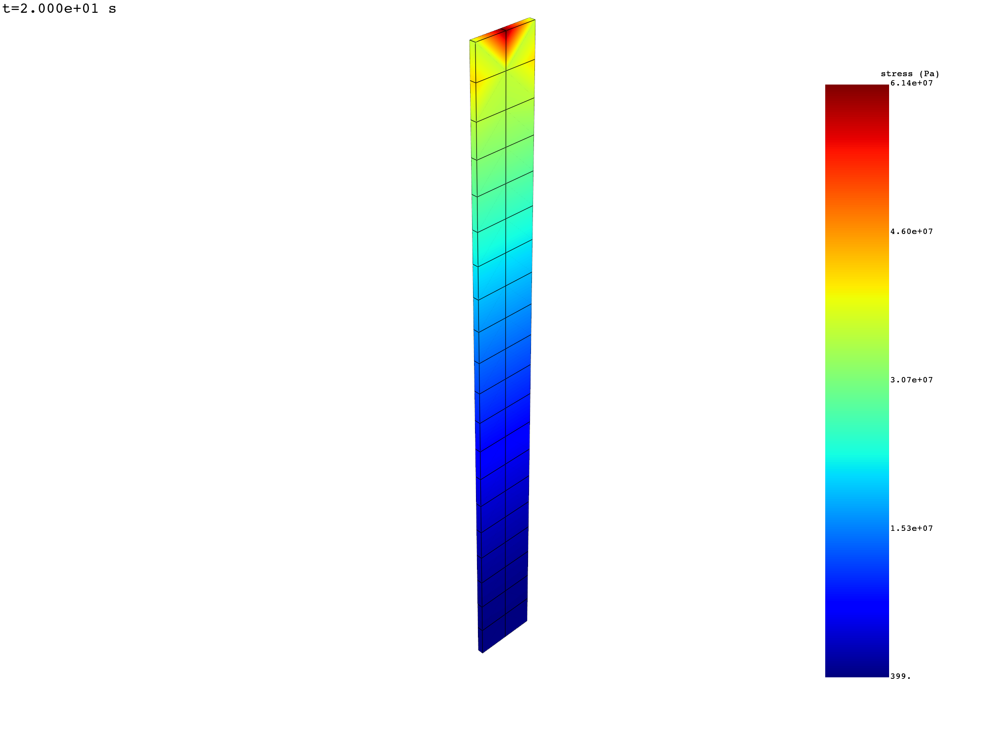
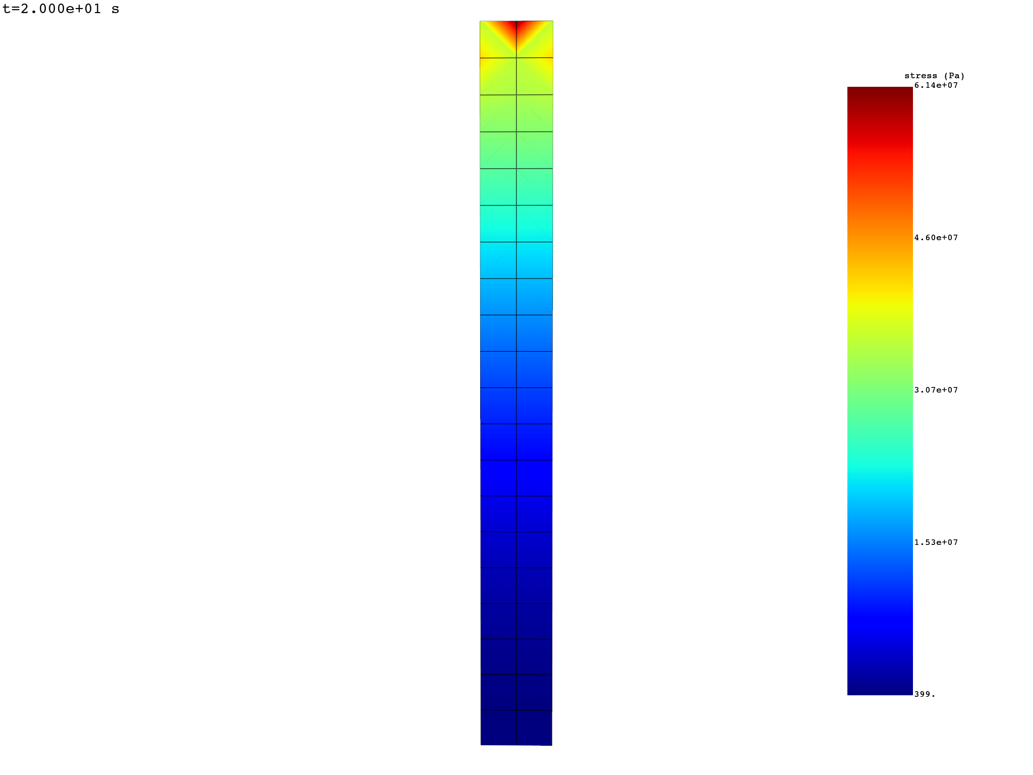
Animate the stress — static mesh

stress_fc.animate()

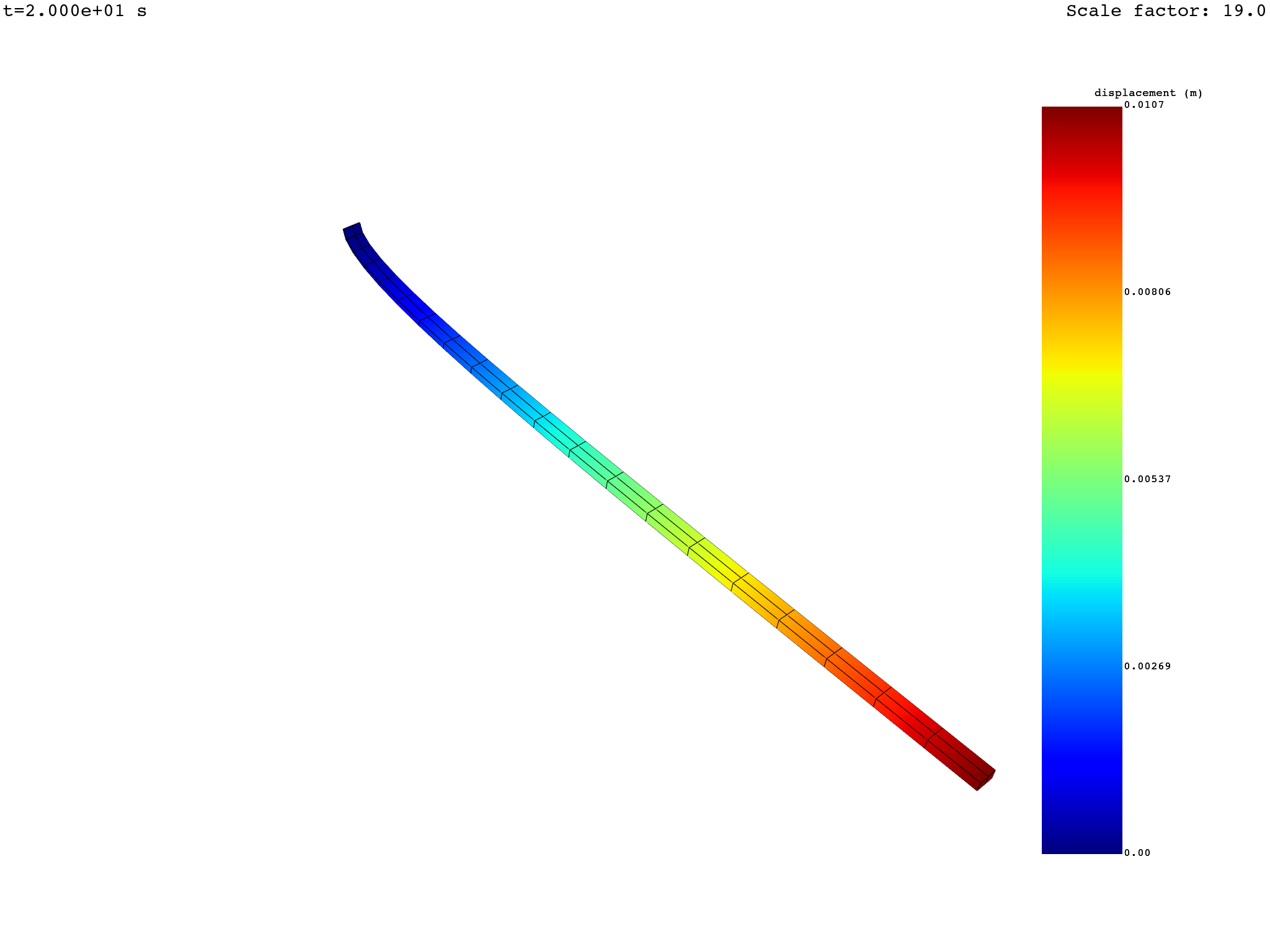
Change the scale factor

The scale factor can be:

• A single number for uniform constant scaling.

• A list of numbers (same length as the number of frames) for varying scaling.

Uniform constant scaling

uniform_scale_factor = 10.0
disp_fc.animate(scale_factor=uniform_scale_factor)

Varying scaling

varying_scale_factor = [float(i) for i in range(len(disp_fc))]
disp_fc.animate(scale_factor=varying_scale_factor)

Save the animation

Use the save_as argument with a target file path. Accepted extensions are .gif, .avi, and .mp4. For more information see pyvista.Plotter.open_movie.

stress_fc.animate(deform_by=disp_fc, save_as="animate_stress.gif")

Control the camera

Control the camera with the cpos argument.

A camera position is a combination of a position, a focal point (target), and an upwards vector:

camera_position = [
    [pos_x, pos_y, pos_z],   # position
    [fp_x, fp_y, fp_z],      # focal point
    [up_x, up_y, up_z],      # upwards vector
]

The animate() method accepts a single camera position or a list of camera positions (one per frame).

Note

A useful technique for defining a camera position: do a first interactive plot with return_cpos=True, position the camera as desired, and retrieve the output of the plotting command.

Fixed camera

cam_pos = [[0.0, 2.0, 0.6], [0.05, 0.005, 0.5], [0.0, 0.0, 1.0]]
stress_fc.animate(cpos=cam_pos)

Moving camera

import copy

cpos_list = [cam_pos]
for i in range(1, len(disp_fc)):
    new_pos = copy.deepcopy(cpos_list[i - 1])
    new_pos[0][0] += 0.1
    cpos_list.append(new_pos)

stress_fc.animate(cpos=cpos_list)

Additional options

You can use additional PyVista arguments, such as:

• show_axes=True / show_axes=False to show or hide the coordinate system axis.

• off_screen=True to render off-screen for batch animation creation.

• framerate to change the frame rate.

• quality to change the image quality.