Note
Go to the end to download the full example code.
Beam results manipulations#
This example provides an overview of the LS-DYNA beam results manipulations.
Note
This example requires DPF 8.0 (DPF 2024 R2) or above. For more information, see Compatibility.
import matplotlib.pyplot as plt

from ansys.dpf import core as dpf
from ansys.dpf.core import examples, operators as ops
d3plot file data extraction#
Create the model and print its contents. This LS-DYNA d3plot file contains several individual results, each at different times. The d3plot file does not contain information related to Units.
In this case, as the simulation was run through Mechanical, a ‘’file.actunits’’ file is produced. If this file is supplemented in the data_sources, the units will be correctly fetched for all results in the file as well as for the mesh.
d3plot = examples.download_d3plot_beam()
my_data_sources = dpf.DataSources()
my_data_sources.set_result_file_path(d3plot[0], key="d3plot")
my_data_sources.add_file_path(d3plot[3], key="actunits")
my_model = dpf.Model(my_data_sources)
print(my_model)
DPF Model
------------------------------
Unknown analysis
Unit system: Custom: mm, ton, N, s, mV, mA, degC
Physics Type: Unknown
Available results:
     -  global_kinetic_energy: TimeFreq_steps Global Kinetic Energy
     -  global_internal_energy: TimeFreq_steps Global Internal Energy
     -  global_total_energy: TimeFreq_steps Global Total Energy
     -  global_velocity: TimeFreq_steps Global Velocity
     -  initial_coordinates: Nodal Initial Coordinates
     -  coordinates: Nodal Coordinates
     -  velocity: Nodal Velocity
     -  acceleration: Nodal Acceleration
     -  stress: Elemental Stress
     -  stress_von_mises: Elemental Stress Von Mises
     -  plastic_strain_eqv: Elemental Plastic Strain Eqv
     -  total_strain: Elemental Total Strain
     -  beam_axial_force: Elemental Beam Axial Force
     -  beam_s_shear_force: Elemental Beam S Shear Force
     -  beam_t_shear_force: Elemental Beam T Shear Force
     -  beam_s_bending_moment: Elemental Beam S Bending Moment
     -  beam_t_bending_moment: Elemental Beam T Bending Moment
     -  beam_torsional_moment: Elemental Beam Torsional Moment
     -  beam_axial_stress: Elemental Beam Axial Stress
     -  beam_rs_shear_stress: Elemental Beam Rs Shear Stress
     -  beam_tr_shear_stress: Elemental Beam Tr Shear Stress
     -  beam_axial_plastic_strain: Elemental Beam Axial Plastic Strain
     -  beam_axial_total_strain: Elemental Beam Axial Total Strain
     -  history_variablesihv__[1__10]: Elemental History Variables(ihv: [1, 10])
     -  displacement: Nodal Displacement
------------------------------
DPF  Meshed Region:
  1940 nodes
  2056 elements
  Unit: mm
  With solid (3D) elements, beam (1D) elements
------------------------------
DPF  Time/Freq Support:
  Number of sets: 12
Cumulative     Time (s)       LoadStep       Substep
1              0.000000       1              1
2              0.997460       2              1
3              1.997818       3              1
4              2.998237       4              1
5              3.998657       5              1
6              4.999076       6              1
7              5.999496       7              1
8              6.999915       8              1
9              7.997509       9              1
10             8.997929       10             1
11             9.998348       11             1
12             10.001174      12             1
Exploring the mesh#
The model has solid (3D) elements and beam (1D) elements. Some of the results only apply to one type of elements (such as the stress tensor for solids, or the axial force for beams, for example).
By splitting the mesh by element shape we see that the ball is made by the solid 3D elements and the plate by the beam 1D elements
Define the analysis mesh
my_meshed_region = my_model.metadata.meshed_region

# - Get separate meshes for each body
my_meshes = ops.mesh.split_mesh(
    mesh=my_meshed_region, property=dpf.common.elemental_properties.element_shape
).eval()

# - Define the meshes for each body in separate variables
ball_mesh = my_meshes.solid_mesh(label_space={"body": 1})
plate_mesh = my_meshes.beam_mesh(label_space={"body": 2})

print(my_meshes)
DPF  Meshes Container
  with 2 mesh(es)
  defined on labels: body elshape

  with:
  - mesh 0 {body:  1, elshape:  2, } with 1651 nodes and 1512 elements.
  - mesh 1 {body:  2, elshape:  3, } with 289 nodes and 544 elements.
Plate mesh
print("Plate mesh", "\n", plate_mesh)
plate_mesh.plot(title="Plate mesh", text="Plate mesh")
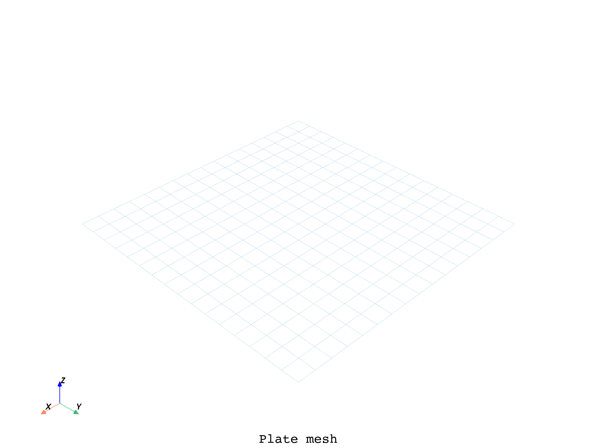
Plate mesh
 DPF  Meshed Region:
  289 nodes
  544 elements
  Unit: mm
  With beam (1D) elements

([], <pyvista.plotting.plotter.Plotter object at 0x0000023EC8720110>)
Ball mesh
print("Ball mesh", "\n", ball_mesh, "\n")
ball_mesh.plot(title="Ball mesh", text="Ball mesh")
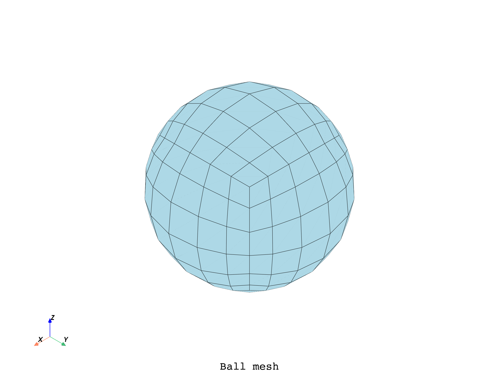
Ball mesh
 DPF  Meshed Region:
  1651 nodes
  1512 elements
  Unit: mm
  With solid (3D) elements


([], <pyvista.plotting.plotter.Plotter object at 0x0000023EE379C210>)
Scoping#
Define the mesh scoping to use it with the operators
my_meshes_scoping = ops.scoping.split_on_property_type(mesh=my_meshed_region).eval()
Define the mesh scoping for each body/element shape in separate variables
ball_scoping = my_meshes_scoping.solid_scoping()
plate_scoping = my_meshes_scoping.beam_scoping()
We will plot the results in a mesh deformed by the displacement. The displacement is in a nodal location, so we need to define a nodal scoping for the plate
plate_scoping_nodal = dpf.operators.scoping.transpose(
    mesh_scoping=plate_scoping, meshed_region=my_meshed_region
).eval()
Beam results#
The next manipulations can be applied to the following beam operators that handle the correspondent results :
beam_axial_force: Beam Axial Force
beam_s_shear_force: Beam S Shear Force
beam_t_shear_force: Beam T Shear Force
beam_s_bending_moment: Beam S Bending Moment
beam_t_bending_moment: Beam T Bending Moment
beam_torsional_moment: Beam Torsional Moment
beam_axial_stress: Beam Axial Stress
beam_rs_shear_stress: Beam Rs Shear Stress
beam_tr_shear_stress: Beam Tr Shear Stress
beam_axial_plastic_strain: Beam Axial Plastic Strain
beam_axial_total_strain: Beam Axial Total Strain
We do not demonstrate separately how to use each of them in this example once they have similar methods.
So, if you want to operate on other operator, uou just need to change their scripting name in the code lines.
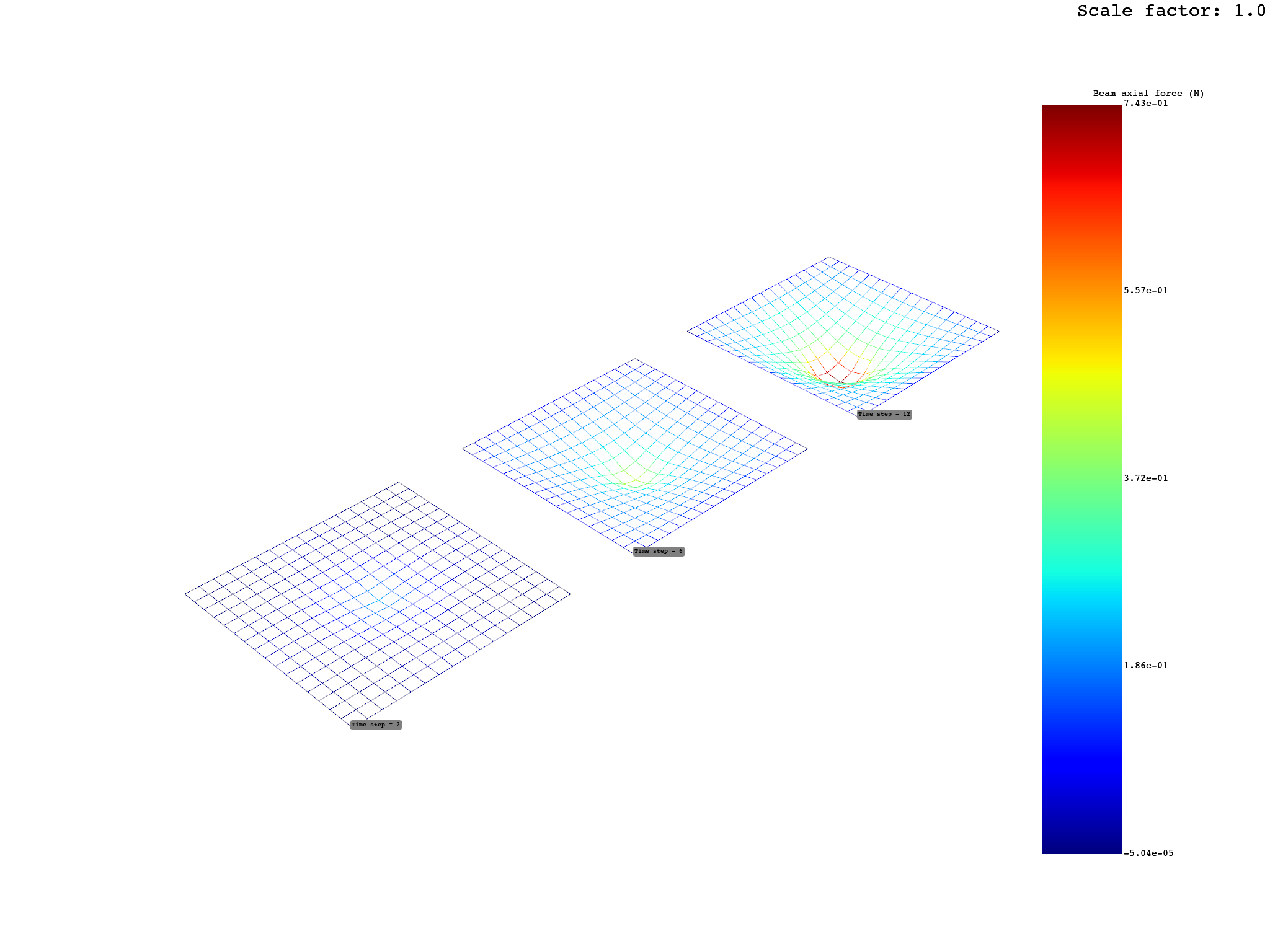
Comparing results in different time steps#
# 1) Define the time steps set
time_steps_set = [2, 6, 12]

# 2) Prepare the collections to store the results for each time step

#    a. To compare the results in the same image you have to copy the mesh for each plot
plate_meshes = dpf.MeshesContainer()
plate_meshes.add_label("time")

#    b. The displacements for each time steps to deform the mesh accordingly
plate_displacements = dpf.FieldsContainer()
plate_displacements.add_label(label="time")

#   c. The axial force results for each time steps. Here
plate_axial_force = dpf.FieldsContainer()
plate_axial_force.add_label(label="time")

# 3)  Use the Plotter class to add the plots in the same image
comparison_plot = dpf.plotter.DpfPlotter()

#   Side bar arguments definition
side_bar_args = dict(
    title="Beam axial force (N)", fmt="%.2e", title_font_size=15, label_font_size=15
)

# 4) As we want to compare the results in the same plot we will need this variable.
# It represents the distance between the meshes
j = -400

# 5) Copy the mesh of interest. Here it is the plate mesh that we copy along the X axis
# Here we use a loop where each iteration correspond to the manipulations for a given time step

for i in time_steps_set:  # Loop through the time steps
    # Copy the mesh
    plate_meshes.add_mesh(label_space={"time": i}, mesh=plate_mesh.deep_copy())

    # 6) Get the plot coordinates that will be changed (so we can compare the results side by side)
    coords_to_update = plate_meshes.get_mesh(
        label_space_or_index={"time": i}
    ).nodes.coordinates_field

    # 7) Define the coordinates where the new mesh will be placed
    overall_field = dpf.fields_factory.create_3d_vector_field(
        num_entities=1, location=dpf.locations.overall
    )
    overall_field.append(data=[j, 0.0, 0.0], scopingid=1)

    # 8) Define the updated coordinates
    new_coordinates = ops.math.add(fieldA=coords_to_update, fieldB=overall_field).eval()
    coords_to_update.data = new_coordinates.data

    # 9) Extract the result, here we start by getting the beam_rs_shear_stress
    plate_axial_force.add_field(
        label_space={"time": i},
        field=my_model.results.beam_axial_force(
            time_scoping=i, mesh_scoping=plate_scoping_nodal
        ).eval()[0],
    )
    # 10) We will also get the displacement to deform the mesh
    plate_displacements.add_field(
        label_space={"time": i},
        field=my_model.results.displacement(
            time_scoping=i, mesh_scoping=plate_scoping_nodal
        ).eval()[0],
    )
    # 11) Add the result and the mesh to the plot
    comparison_plot.add_field(
        field=plate_axial_force.get_field(label_space_or_index={"time": i}),
        meshed_region=plate_meshes.get_mesh(label_space_or_index={"time": i}),
        deform_by=plate_displacements.get_field(label_space_or_index={"time": i}),
        scalar_bar_args=side_bar_args,
    )
    comparison_plot.add_node_labels(
        nodes=[289],
        labels=[f"Time step = {i}"],
        meshed_region=plate_meshes.get_mesh(label_space_or_index={"time": i}),
        font_size=10,
    )
    # 12) Increment the coordinate value for the loop
    j = j - 400


# Visualise the plot
comparison_plot.show_figure()
([], <pyvista.plotting.plotter.Plotter object at 0x0000023ED8CB5110>)
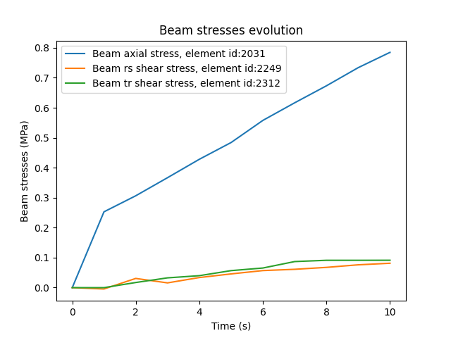
Plot a graph over time for the elements with max and min results values#
Here we make a workflow with a more verbose approach. This is useful because we use operators having several matching inputs or outputs. So the connexions are more clear, and it is easier to use and reuse the workflow.
The following workflow finds the element with the max values over all the time steps and return its ID
# Define the workflow object
max_workflow = dpf.Workflow()
max_workflow.progress_bar = False
# Define the norm operator
max_norm = ops.math.norm_fc()
# Define the max of each entity with the evaluated norm as an input
max_per_ent = ops.min_max.min_max_by_entity(fields_container=max_norm.outputs.fields_container)
# Define the max over all entities
global_max = ops.min_max.min_max(field=max_per_ent.outputs.field_max)
# Get the scoping
max_scop = ops.utility.extract_scoping(field_or_fields_container=global_max.outputs.field_max)
# Get the id
max_id = ops.scoping.scoping_get_attribute(
    scoping=max_scop.outputs.mesh_scoping_as_scoping, property_name="ids"
)

# Add the operators to the workflow
max_workflow.add_operators(operators=[max_norm, max_per_ent, global_max, max_scop, max_id])
max_workflow.set_input_name("fields_container", max_norm.inputs.fields_container)
max_workflow.set_output_name("max_id", max_id.outputs.property_as_vector_int32_)
max_workflow.set_output_name("max_entity_scoping", max_scop.outputs.mesh_scoping_as_scoping)
Using the workflow to the stresses results on the plate:
Extract the results
# Get all the time steps
time_all = my_model.metadata.time_freq_support.time_frequencies

# Extract all the stresses results on the plate
plate_beam_axial_stress = my_model.results.beam_axial_stress(
    time_scoping=time_all, mesh_scoping=plate_scoping
).eval()
plate_beam_rs_shear_stress = my_model.results.beam_rs_shear_stress(
    time_scoping=time_all, mesh_scoping=plate_scoping
).eval()
plate_beam_tr_shear_stress = my_model.results.beam_tr_shear_stress(
    time_scoping=time_all, mesh_scoping=plate_scoping
).eval()
As we will use the workflow for different results operators we group them and use a loop through the group. Here we prepare where the workflow outputs will be stored
# List of operators to be used in the workflow
beam_stresses = [plate_beam_axial_stress, plate_beam_rs_shear_stress, plate_beam_tr_shear_stress]
graph_labels = [
    "Beam axial stress",
    "Beam rs shear stress",
    "Beam tr shear stress",
]

# List of elements ids that we will get from the workflow
max_stress_elements_ids = []

# Scopings container
max_stress_elements_scopings = dpf.ScopingsContainer()
max_stress_elements_scopings.add_label("stress_result")
- The following loop:
Goes through each stress result and get the element id with maximum solicitation
Re-escope the fields container to keep only the data for this element
Plot a stress x time graph
for j in range(0, len(beam_stresses)):  # Loop through each stress result
    # Use the pre-defined workflow to define the element with maximum solicitation
    max_workflow.connect(pin_name="fields_container", inpt=beam_stresses[j])
    max_stress_elements_ids.append(
        max_workflow.get_output(pin_name="max_id", output_type=dpf.types.vec_int)
    )
    max_stress_elements_scopings.add_scoping(
        label_space={"stress_result": j},
        scoping=max_workflow.get_output(
            pin_name="max_entity_scoping", output_type=dpf.types.scoping
        ),
    )

    # Re-scope the results to keep only the data for the identified element
    beam_stresses[j] = ops.scoping.rescope_fc(
        fields_container=beam_stresses[j],
        mesh_scoping=max_stress_elements_scopings.get_scoping(
            label_space_or_index={"stress_result": j}
        ),
    ).eval()

    # The d3plot file gives us fields containers labeled by time. So in each field we have the stress value in a
    # given time for the chosen element. We need to rearrange the fields container into fields.

    beam_stresses[j] = ops.utility.merge_to_field_matrix(fields1=beam_stresses[j]).eval()
    plt.plot(
        time_all.data,
        beam_stresses[j].data[0],
        label=f"{graph_labels[j]}, element id:{max_stress_elements_ids[j][0]}",
    )

# Graph formatting
plt.title("Beam stresses evolution")
plt.xlabel("Time (s)")
plt.ylabel("Beam stresses (MPa)")
plt.legend()
plt.show()
Results coordinates system#
The general results are given in the Cartesian coordinates system by default.
The beam results are given directly in the local directions as scalars. For example the beam stresses we have:
The axial stress, given in the beam axis
The stresses defined in the cross-section directions: tr stress in the transverse direction (t) and rs stress perpendicular to the tr direction (s).
Unfortunately there are no operators for LS-DYNA files that directly allows you to: - Rotate results from local coordinate system to global coordinate system; - Extract the rotation matrix between the local and global coordinate systems;
Total running time of the script: (0 minutes 10.733 seconds)